Data Structure
view on github- Introductions
- Asymptotic Complexity
- Abstract Data Type(ADT)
- Priority Queue(PQ)
- Recurrence
- Sort
- Hashing
- Dictionary ADT
- Problems with Direct-Addressed Tables
- When keys Collide
- A Simple Strategy: Chaining
- Performance of Hash Table
- Simple Uniform Hashing (SUH)
- Hash Function Pipeline - Second Steps
- Divsion Mapping
- Multiplicative Hashing
- Open Address Hashing
- Purpose of Hashcode Generation
- Hashing Composite Objects
- Binary Search Trees(Lecture 10)
- AVL Tree and B+ Tree
- Graph
- Weighted Shortest Paths
- Weighted Shortest Paths
- Greedy Algorithm and the Minimum Spanning Tree
Recommended Books
Introductions
Algorithm Definition
- An “Effective Procedure”
- For taking any instance of a computational problem
- finding a correct solution
Asymptotic Complexity
Desirable Properties of Running Time Estimates
Definition of Big-O Notation
we say that $f(n)=O(g(n))$ if exists constants
\[c>0, n_0>0\]such that for all $n\geq{n_0}$
\[f(n)\leq{c\cdot{g(n)}}\]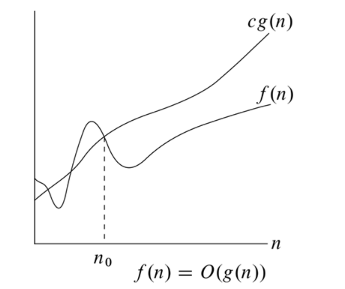
- Big-O Ignores Constants, as Desired
- Lemma: If $f(n)=O(g(n))$, then $f(n)=O(a\cdot{g(n)}),\ \forall{a>0}$
- Pf: Since we know $f(n)=O(g(n)) \Rightarrow{f(n)\leq{cg(n)}}$, and we have $f(n)\leq{\frac{c}{a}\cdot{a}g(n)}$
- Conclude that $f(n)=O(g(n))$ $\textbf{QED}$
- General Strategy for Proving $f(n)=O(g(n))$
- Pick $c>0$, $n_0>{0}$
- Write down desired inequalities $f(n)\leq{cg(n)}$
- Solve inequalities to find out constant $c$ to hold it whenever $n\geq{n_0}$
- Generalization of Previous Proof
- Therom: Any polynomial of the form $s(n)=\sum_{j=0}^{k}{a_{j}n^{j}}$ is $O(n^{k})$
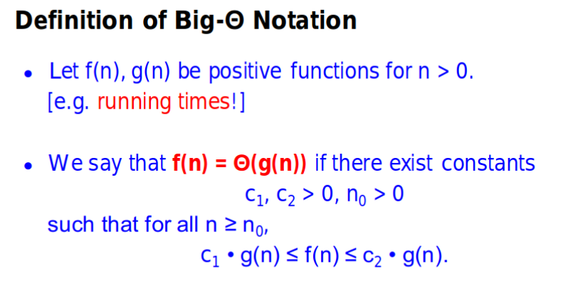
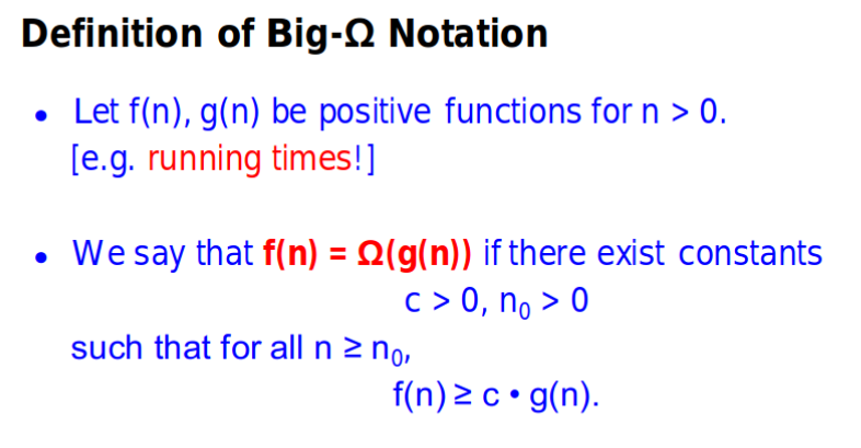
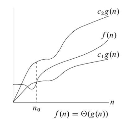
Defintion of Big-$\Omega$, $\Theta$
Small o, $\omega$ notation
- Small o, if $f(n)=O(g(n))$ but $f(n)\neq{\Omega(g(n))}$
- Small $\omega$, if $f(n)=\Omega(g(n))$ but $f(n)\neq{O(g(n))}$
- Big $\Theta$, if $f(n)=\Omega(g(n))$ and $f(n)={O(g(n))}$
- IN SUMMARY
- $0$, $f(n)=o(g(n))$
- $\infty$, $f(n)=\omega{(g(n))}$
- $k>0$, $f(n)=\Theta(g(n))$
- Tips for derivative formula:
Some other conclusions
- Exponentials Grows faster than Polynomials
Abstract Data Type(ADT)
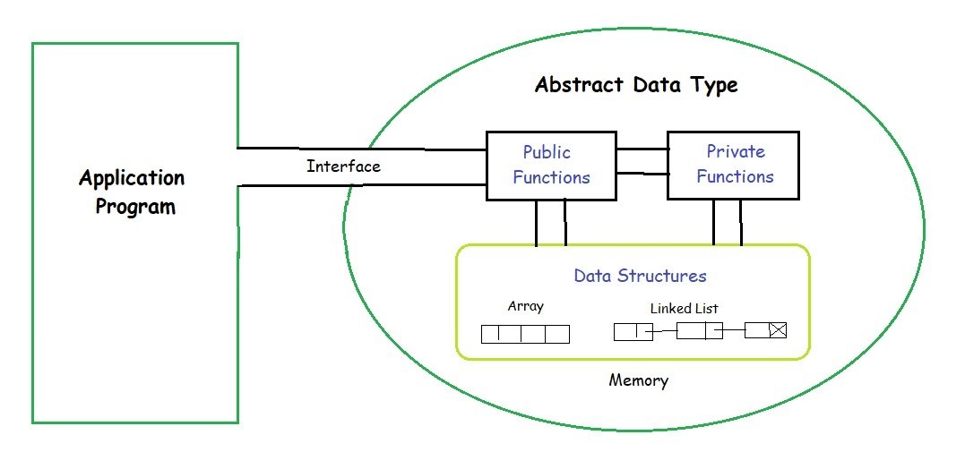
The definition of ADT only mentions what operations are to be performed but not how these operations will be implemented. It does not specify how data will be organized in memory and what algorithms will be used for implementing the operations. It is called “abstract” because it gives an implementation-independent view. The process of providing only the essentials and hiding the details is known as abstraction.(Copied From GeeksforGeeks)
- The simplest way to explain this is:
- We choose an ADT with some required time complexity methods;
- And we choose certain physical data structure to create a certain data structure(ordered list; ordered array; binary tree; heap;)
- For example:
- We need a priority queue(which is a kind of queue), and we can use ordered list or heap(by array) to implement those methods. With consideration of time complexity, we may choose heap.
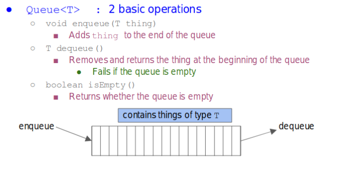
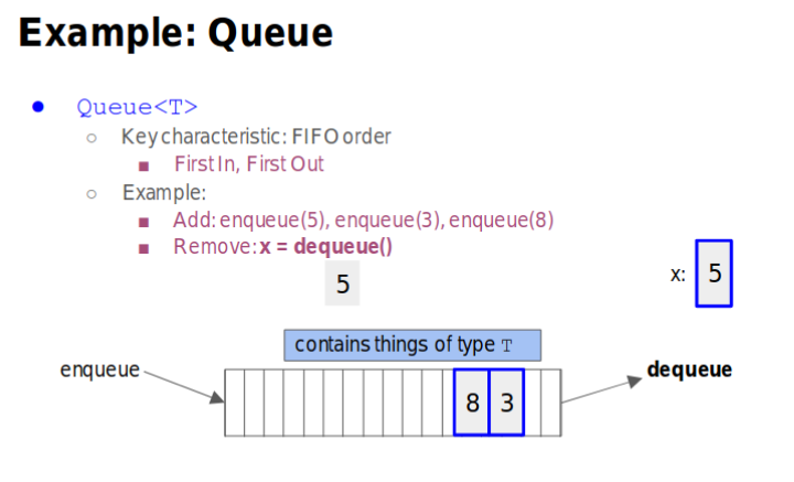
Queue
- enqueue(): Add thing to the end of the queue
- dequeue(): Removes and returns thing at the beginning og the queue
- isEmpty(): Return whether the queue is empty
- First In First Out(FIFO)
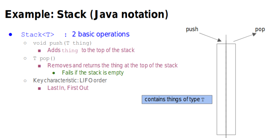
Stack
- push(): Adds thing to the top of the stack
- pop(): Removes and Returns the thing at the top of the stack
- Last In First Out(LIFO)
An ADT can be implemented in different ways
- Example: Queue implemented by array
- Idea: Maintain Head, Tail pointers
- Enqueue items at the tail
- Dequeue items at the head
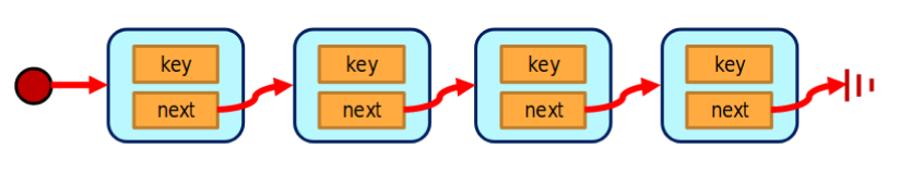
Linked List
- Add Pointers to Queue
- Tail Pointer for enqueue()
- Head Pointer for dequeue()
- Each Pointers of Nodes points to next Nodes
- The last Node next pointer is null
- Relative: Studio2.Linklists
- Links to understand
- AddLast Function
- Use Pointer p do p.next loop to find p.next==null, then make p.next = q
while(p.next!=null){
    p = p.next;
}
p.next = q;
SUMMARY for Queue and Stack
Queue: Add to tail; Remove from the head;
Stack: Add to top; Remove from the top;
Priority Queue(PQ)
Priority Queue Default
- In PQ, we assume that the header items is the min value
- Therefore, extractMin() method will cost you $\Theta(n)$
- Ideas?
- Unsorted List: High cost for second min value after extractMin()
- Sorted List: High cost for insert
- Unsorted Array: Just the same as unsorted list
- Since these are high for list, we need a new data structure to meet better than $\Theta(n)$ for extraction and insertion.
Heap
-
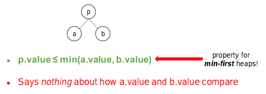
A binary heap is a compact binary tree with an ordering invariant –the heap property.
-
Heap property: a special relationship between each parent and its children.
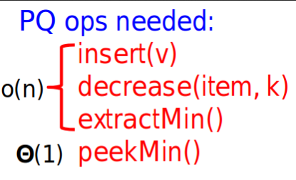
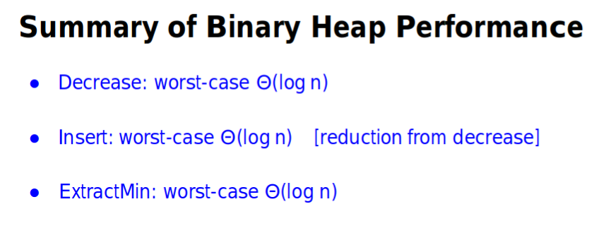
- Several Operations for Heap
- Insert()
- Extractmin()
- Decrease()
- Decrease()
- Decrease the certain number
- Change position with Parent if necessary
- Insert()
- Just the same as Decrease()
- Extractmin()
- After extract the root, Heap is no longer compact
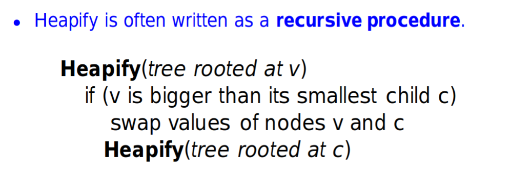
- We need to rearrange the order with heapify()
- Heapify()
- Move the last leaf node(highest rightest leaf node) to root
- Change position if necessary
- Theorm1
- A complete binary tree of height $k$ has $2^{k+1}-1$ nodes. (First height level is 0)
- Means: has $2^{k}$ nodes.
- Therefore, a complete binary tree has height of $\log_{2}(n)$
- Conclusion:
- Accroding to Theorm1, we can conclude that decrease/insert/heapify has time complexity of $\log_{2}(n)$.
- Another way to analyze complexity
- Let’s consider about the worst situation
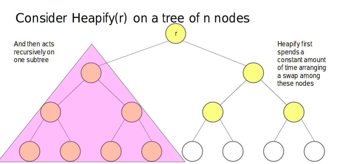
- The nodes in shade $\leq{\frac{2n}{3}}$ for whole trees.
- If the tree has height of $h$, thus we will have $2^{h+1}-1-2^{h-1}$ nodes
- Then the nodes in shade will be $2^{h}-1$
- Therefore, we can say that
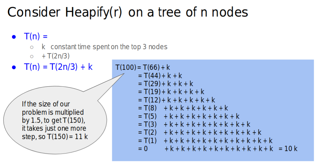
- Thus this give us that $T(n)=\Theta(\log(n))$
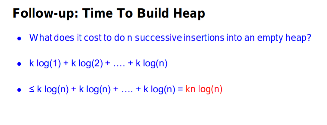
- Follow Up: Time to Build a Heap
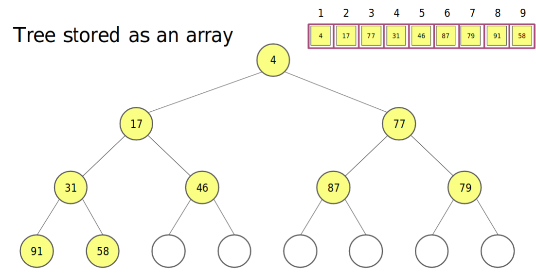
- But in practice, we do not store our heap as a tree
- If P(parent node) is in index $i$
- Then P childrens will be located in $2i$ and $2i+1$
- In reverse, if the C(Child node) is in index $n$
- Then his parent node will be located in $[\frac{n}{2}]$
Look back to compare different Implementations
-
Binary Heap
-
List
- Link vs Array
- Sorted vs Unsorted
| Implementation | insert | extractMin |
|---|---|---|
| Unordered List | $\Theta(1)$ | $\Theta(n)$ |
| Ordered List | $\Theta(n)$ | $\Theta(1)$ |
| Unordered Array | $\Theta(1)$ | $\Theta(n)$ |
| Ordered Array | $\Theta(n)$ | $\Theta(1)$ |
- We can use binary search in Ordered Array to find where to insert but we still need $\Theta(n)$ time to rearrange the array. Therefore $\Theta(n)+\Theta(\log{n})+\Theta(1)=\Theta(n)$
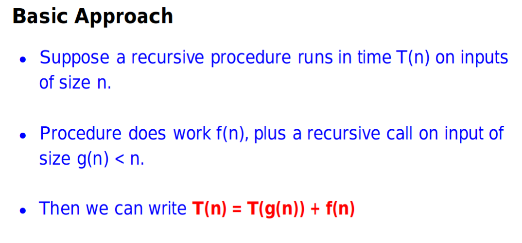
Recurrence
Substituion(Guess and Check)
- Claim and then math induction
Recurrence Table
- Bianry Search $T(n)=T(\frac{n}{2})+c$
-
Merge Sort $T(n)=2T(\frac{n}{2})+cn$
- Create table with following features:
- Depth
- Problem Size
- Node per Level
- Local Work Per Node
- Local Work Per Level
Master Theorem
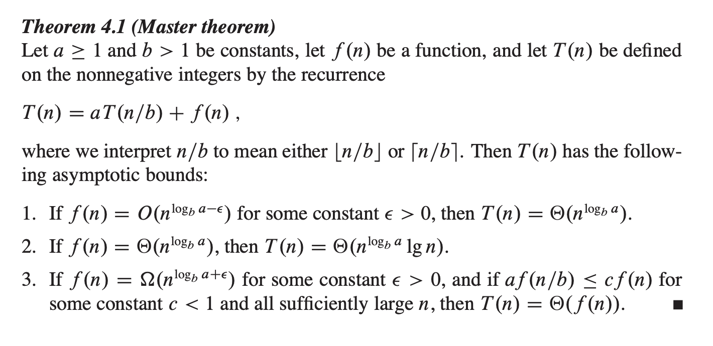
Also, Master Theorem in wikipedia has explanation on this.
Binary Search
- Binary Search Recurrence
Sort
Comparison Sort
- We want a lower bound for comparison sort algorithm
- How many comparisons do we need to sort an input array of size n?
- A trivial lower bound $\Omega(n)$
- And improve this lower bound
- It is impossible to sort in time in less than $n{\log}n$ (Using comparisons)
- Let’s see how we can sort in time less than nlogn(see in radix sort)
Merge Algorithm;
- Sorted Array A, B;
- Fetch Min(A[i], B[j]) into C[k]
Merge Sort Recurrence;
- 2 recurrence, each node n/2;
- 1 Merge() method, local work n;
- $T(n)=2T(\frac{n}{2})+cn$
External Merge Sort
- Introducing video
In Space HeapSort
- The difference between insert() and heapify()
- insert()
- Need to compare its value with its parent, swap if it insert value is smaller.
- This value will go to the place where it should be.(need to be sure that, above this insert value should be a heap.)
- heapify()
- Need to compare its value with its children, swap if children are smaller.
- Make sure this place is min/max value in this heap. (need to be sure that besides the top, below this shuold be a heap.)
- Convert unsorted array into heap without allocating another array(Two Methods)
- Use Heapify(): From the nodes just above the bottom, and traverse to the top of the heap.(Which can make sure that below is a heap).
- Video about this.
- Another video
</br>
- Use Insert(): From the second element, we can just Insert(this_element), which can make sure that above this inserted element is a heap.
- Next Step is to do Heap Sort
- Also this Video talk about this.
- Just swap the 1st element with the last one, and heapify it;
- The swap the 1st element with the second last one, and heapify it with respect to array apart from the last one.
- …
- Finally, we will get an array with order from MAX to MIN.
CountSort
- Input $\Theta(n)$
- Output $\Theta(n+k)$
- Still depends on $k$
- But what if $k$ is large?
RadixSort
- Sort using $d$ successive passes of counting sort
- We sort by least significant digit first
- Sort in each pass must be stable - never inverts order of two inputs with the same key
- Radix buckets using queue(first in first out)
Why does Radix Sort Work?
- Invariant - after $j$ sorting passes, input is sorted by its $j$th least siginificant digits.
- Cost of Radix Sort
- $d$ passes of counting sort
- Total time is $\Theta(d(n+k))$
Hashing
- Is it possible to implement a dictionary with sublinear time for all of insert, remove and find?
Dictionary ADT
- Stores the collection of objects
- Each objects is associated with a key
- Objects can be dynamically inserted and removed
- Can efficiently find an object in the dictionary by its key
Problems with Direct-Addressed Tables
- What if $|U|»n$;
- What if keys are not integers?
When keys Collide
- What happen if multiple keys hash to same table cell
- This must happen if $m<|U|$ – pigeonhole principle
- When two keys hash to same cell, we say they collide.
A Simple Strategy: Chaining
- Each table cell becomes a bucket that can hold multiple records
- A bucket holds a list of all records whose keys map to it
Performance of Hash Table
- “Performance” = “cost to do a find()”
- Tips: insert; delete, similarly traverse list for some bucket
- For insert, you have to make sure that this value is unique in this bucket, which need to traverse the list;
- For delete, you need to find this element first, and delete it.
- In worst case, all n records hash to one bucket.
- Thus, we get $\Theta(n)$ for all of these cases.
Simple Uniform Hashing (SUH)
- Assume that, given a key in U, hash function is equally like to map k into each value $[0,m)$, independent of all other keys.
- Then we get the average cost of search for this $\frac{n}{m}$, where $m$ is the number of buckets.
- Plus $\Theta(1)$ for computing the hash code.
At here, we define the load factor with:
\[\alpha=\frac{n}{m}\]Hash Function Pipeline - Second Steps
- Given a hashcode, where should we put it to certain bucket?
- Assumptions:
- Hashcodes are in range $[0,N)$
- Need to convert hashcodes to indices in $[0,m)$
- $m$ is the table size
Divsion Mapping
- b(c) = c mod m
- Perils of Division Hashing
- Claim: if j = c mod m, then j mod d = c mod d;
- E.g, if d = 2, then even hashcodes map to even indices, do not map uniformly across the entire table => not SUH behaviour!
- A particular bad case:
- Suppose we get $m=2^v$, and mod $m$ just always the bits pattern in last $v$ bits
- Advice on Division Hashing
- $m$ has no obvious correlations between hashcode bit pattern and index
- Idea: make $m$ a prime number
- What is wrong with $m$ near Power of 2 or 10
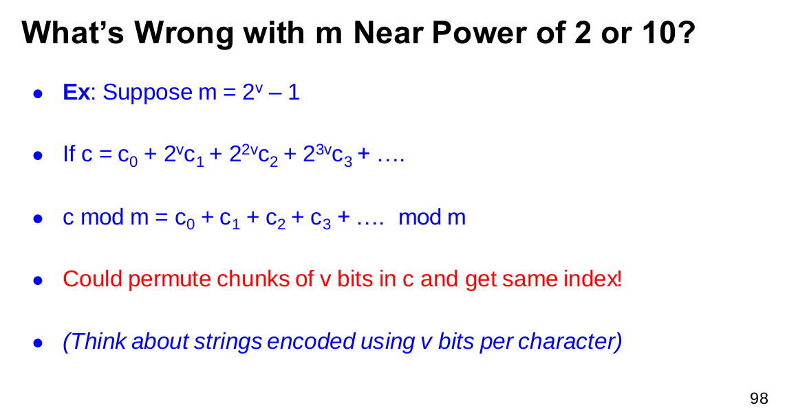
we can make an example to try this:
\[\begin{aligned} 2^{2v}\cdot{c_2} \ mod\ (2^v-1) &=2^v\cdot2^vc_2\ mod\ (2^v-1) \\ &=2^v[(2^v-1)c_2+c_2]\ mod\ (2^v-1)\\ &=c_2\ mod\ (2^v-1) \end{aligned}\]Multiplicative Hashing
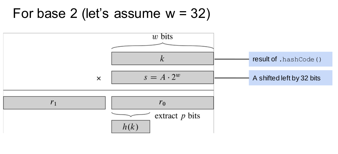
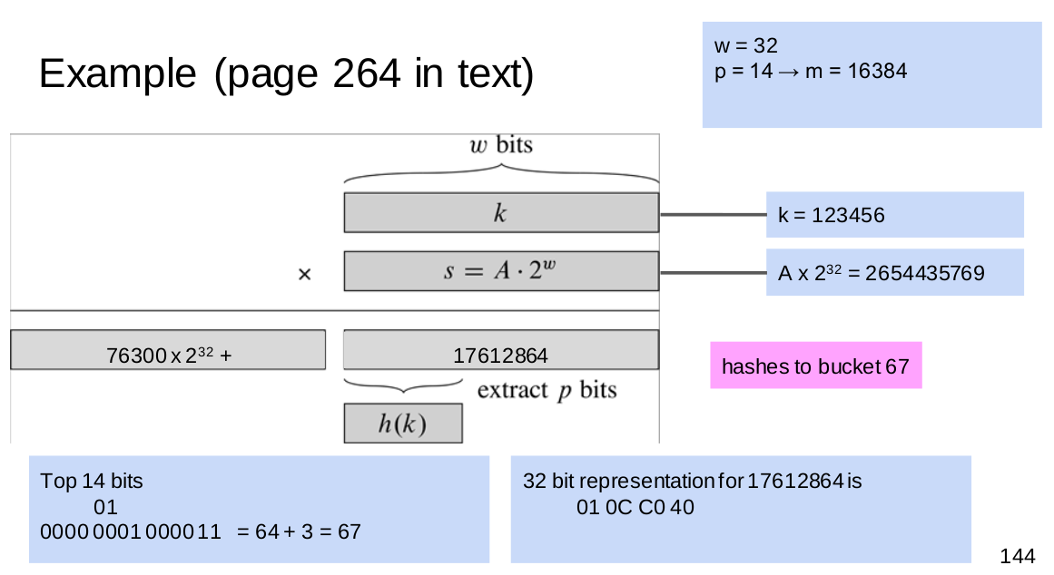
\[b(c) = (c\cdot{A}\ mod\ 1.0)\cdot{m}\]-
cA mod 1.0 is in [0, 1), so b(c) is an integer in [0,m)- an index
-
In particular, we can use $m=2^v$ if we want.
- Some choice of A is also not good, like:
- 0.75, with so zeros after 5;
- 7/9=0.7777777… have poor diffusion
- ex: $A=\frac{\sqrt{5}-1}{2}$
- For base2, we certainly will get
Open Address Hashing
-
A chained hash table needs two data structures:
-
Notes on open addressing:
- Maintain load factor $\alpha=\frac{n}{m}<1$
- Average search time $\Theta(\frac{1}{1-\alpha})$
- we want a larger $m$
- deletion is harder
- deletion must leave behind a “deleted” marker so find does not stop prematurely
Purpose of Hashcode Generation
- Map objects to integers in some range
- Objects equals() have some hashcode
- Q: should hashcodes be spread uniformly accross range without obvious correlations?
- No, index generation is responsible for uniform;
- Yes, index generation is not responsible for “fixing” a bad hashcode.
- Java: No, hashcodes do not need be uniform and correlated;
-
C++: Yes.
-
But if universe of objects is much bigger than #possible hashcodes, the non-uniformity, correlations increase the likelihood that you will encounter many objects that map to the same hashcode.
- Hashcode Ideas for Primitive Types
- 32 bit integer;
- 32 floating point - floatToIntBits()
-
64 bits long (including double precision float via doubleToLongBits())
- Problems:
- Types with limited #of values;
- Mapping with “nice” properties
- E.g. Boolean: true->1231; false->1237;
Hashing Composite Objects
- Sets:
- summation;
- mimimum;
- Sequences
- using prime number to time its order;
- 31 is small, and can add more small hashcodes w/o overflowing;
-
But it is still easy to find many short sequences that map to same hashcode!
- Example Alternative: Fowler-Noll-Vo-Hashing
- c <- (c XOR cj)*16777619;
- $16777619=2^{24}+2^8+147$
Binary Search Trees(Lecture 10)
- Motivation – limitation of dictionaries
- Hash has at least two undesirable limitations
- Worst-case op $\Theta(n)$
- Do not adequately naturally ordered collections
- Ordered Dynamics Set Operations
- max/min
- iterator
- Would like Sub-linear time insert/remove/find
Binary Search Tree
- BST invariants:
- x.left <= x;
- x >= x.right;
Find: Use BST Property
- Suppose we want to search k with tree rooted at node x
- If k < x, search in left;
- If k > x, search in right;
- Else k == x, we are done!
- MIN/MAX
- Most left would be the MIN;
- Most right would be the MAX;
Insertion
- Use find to get to the null leaf, which will be the position for node to insert;
Iteration
- Successor
- If x has a right subtree T’, return leftmost of T’
- If has no right subtree, then x will be the maximum node as subtree T for some node y. (follow parent pointers until some node y is a right parent)
Remove
- If x is a leaf;
-
If x has one subtree, remove x and link subtree’s root to x’s parent;
- REMOVE a node x with 2 subtrees
- replace x with succ(x)=y
- then delete node y
- (Will have at most two deletions)
What if our trees were never too tall?
-
In a balanced BST, all operations in worst case are $O(\log{n})$
-
An example of balanced property: AVL tree
- Defn: T is an AVL tree iff, for every node x in T, one of these is true:
- x is a leaf
- x has one child, which is a leaf
- x has two children, |x.right.h - x.left.h| <= 1
- Why AVL trees are balanced?
- In worst case, $N(h)=N(h-1)+N(h-2)$
- Claim: AVL tree at least has $\Phi^{h}$ nodes
AVL Tree and B+ Tree
Check AVL Property
- Key measurement: Balance Factor
- x.right.h - x.left.h
- How to maintain height(Studio 10 Part C)
Tree Rotation
- Right Rotation
- Case1: left left is heavier: right rotation
- Case2: left right is heavier: left rotation; right rotation
When do we rebalance?
- Inserting or removing nodes in some place, we may want to rebalance each ancestor of x moving up the tree.
- Insertions: safe after first rebalancing;
- Deletions: must continue and check rebalancing until root
2-3-4 Trees
-
Every path from root to the bottom of the tree has same height
- Probelm with insertion
- Split the leaf
- Can generalize 2-3-4 trees to B-trees
- Red-Black Trees
- Deletion Probelm(Studio 11)
Graph
Some definitions of Graph
-
A graph $G=(V,E)$ is a set of nodes or vertices, together with a set of $E$ of edges(described as pairs of vertices)
-
How do we represent graphs in a computer?
-
Exploration - Graph Traversals
BFS
- Algorithm
- Using Queue to record those vertices which are marked
- Explore those vertices that in the top of Queue
- Using BFS can just return the shortest path
- A Video about shortest unweighted path implementation from BFS
- A simple reason for this is that if we explore a vertex and whose edge points to a explored vertex, we will not update the distance, since this vertex must have been explored before this edge with shorter path.
- BFS computes shortest path
- Claim: BFS enqueues every vertex $w$ with $D(v,w)=d$ before any vertex $x$ with $D(v,x)>d$.
- Pf: by induction on $d$
- Base($d=0$): $v$ itself is enqueued first and has $D(v,v)=0$
- Ind: consider vertex $w$ with $D(v,w)=d>0$, and there is some $u$ with $D(v,u)=d-1$, and edge $(u,w)$ exists.
- By induction, $u$ will be enqueued and dequeued before $w$. And after $u$ is dequeued, $w$ is enqueued.
- Thus, any vertex with distance $>d$ will be enqueued after $w$.
- Bipartite Testing
- Lemma: If the Graph has a cycle of odd length, then Graph is not bipartite. (Never labels both endpoints of an edge(u,w) with same side.) (No edge that connects vertices of same set.)
- Proof: If it has odd cycle, then we must have combination of LRR or RLL, which means there are two endpoints in the same side. (Slide12 P68, P69)
Deepth First Search(DFS)
- Algorithm
- First Started, Last Finished
- Using implicit stack, and traverse vertex which has not been started yet, and if all edges for this vertex has been started, this algorithm will finish this vertex.
- Cycle Detection
- The method is using: If we find a node has been started, but not yet finished. Then we conclude that this graph contains a cycle.
- Proof is that: Some node $u$ has been started, and now we are at node $w$. If we find that through the path of $w\rightarrow{u}$, we find that $u$ has been started but not yet finished, this means that there is a path $u\rightarrow{w}$.
- Hence, we will conclude that there is a cycle in $u$ and $w$.
- A Video about cycle finding.
Weighted Shortest Paths
Alternate Strategy - “Relaxation”
- Whenever we follow an edge $(v,u)$, check whether
- Algorithm(Dijkstra’s Shortest Path Algorithm)
- At each step, explore edges out of vertex $v$ with smallest $v.dist$, and relax all its adjacent vertices.
- Initialization: starting point with distance 0, and other points with distance $\infty$
- Data Structure: Using Heap with extractMin for key with distance; And insert() + decrease() method for update weighted distance in this Graph
- Correctness of Dijkstra’s Algorithm
- Claim: when we explore the edges out of vertex $v$, $v$ has its correct shortest-path distance $D(start,v)$ stored in current best estimate $v.dist$ (Meaning that this extractMin action is correct for shortest distance for this vertex $v$)
- Pf: by induction on order of exploration
- Base: starting vertex is explored first, with its correct shortest-path distance of 0.
- Ind:
- Assume that $v.dist>D(start,v)$(i.e. v’s distance is wrong with extractMin)
- Let $u$ be last finished(i.e. already explored) vertex on this path. By IH(Induction Hypothesis), $u$ had its correct shortest-path distance when it was explored, and it also has $D(start,u)\leq{D(start,v)}$, since $u$ precedes $v$ on shortest path to $v$.
- And if $u\rightarrow{v}$ is on the shortest path, then exploring $u$’s outgoing edges assigns $v$ its correct shortest-path distance $D(start,v)$. -><-
Implementation
- Initially, every vertex is inserted into PQ w/its starting dist
- Maintain collection of unfinished vertices
- At each step, must efficiently find vertex $v$ in collection by using extractMin with smallest $v.dist$ remove it
- Decreasing $v.dist$ is done by using $v$’s Decreaser object
Weighted Shortest Paths
-
Problem: Given a starting vertex $v$, find path of least total weight from $v$ to each other vertex in the graph.
-
Alternative Strategy - “Relaxation”
- Explore shortest path so far and maintained as $v.dist$
- Whenever we follow an edge(v,u), check whether
- If so, update $u.dist$
Dijsktra’s Shortest Path Algorithm
Using PQ as ADT :
- A little bit like BFS Algorithm
- In heap all vertex first with infty distance
- ExtracMin the smallest one (start vertex)
- Each time traverse all edge for this vertex
- Update(decrease() ) the vertex which can have shorter distance
Correctness of Dijstra Algorithm
- For vertex $v$, if $v.dist\neq{D(Start,v)}$:
- Contradiction: If there are a vertex $u$ on the path from start to $v$, and with IH, we know $u.dist$ is correct, and we find the shortest path from $u$ to $v$, which makes contradiction.
- Otherwise, if there is a vertex $x$ has a distance $x.dist<v.dist$, the extractmin should give $x$ instead of $v$, which also makes contractions.
Greedy Algorithm and the Minimum Spanning Tree
- Want to minimize the total cost to connect all vertices
Minimum Spaning Tree (MST)
- General Idea:
- Without creating cycle
- Pick the edge that is currently best by this criterion
Prim’s Algo
-
Prim’s Criterion: Pick the edge $e$ of minimum $w(e)$ that connects a vertex in T to a vertex not yet in T
- Correctness of Algorithm:
- Claim: After number of edges are chosen, algorithm’s current edge set T is a subset of some minimum spanning tree for G.
- Ind: Suppose Prim’s criterion picks a next edge $e$
- One edge each time with no cycle
- The edge is smallest one (Prim’s Greedy)
- Implementation of Prim’s Algorithm
- Maintain sets of all unconnected vertices
- For each unconnected vertex $v$, maintain $v.conn$ – weight of lowest-weight edge connecting $v$ to any vertex in T
Prim vs Dijsktra
- Prim: shortest weighted path for whole graph
- Dijkstra: shortest weighted path from vertex to vertex
- BFS: shortest path from vertex to vertex
Kruskal Algorithm
- Add to T the edge $e$ of minimum $w(e)$ that does not form a cycle when combined with edges already in T.
- Running Time:
- Sorted edges, run main loop
- Main Loop: Union Find-> Make sure no cycle