Machine Learning with Graphs
view on github- 1. Introduction
- 2. Traditional Methods for ML on Graphs
- 8. Application of Graph Neural Networks
- 9. Theory of Graph Neural Networks
- 10. Heterogenous Graphs and Knowledge Graph Embeddings
- History Papers
- A new model earning in graph domains
- Course Material
- Course CS 224w: Machine Learning with Graphs
- Course Video Link
1. Introduction
1.1 Motivation for Graph ML
- Course Outline
- Tradtional methods: Graphlets, Graph Kernels
- Methods for node embeddings: DeepWalk, Node2Vec
- Graph Neural Network: GCN, GraphSAGE, GAT, Theory of GNNs
- Knowledge graphs and reasoning: TransE, BetaE
- Deep generative models for graphs
- Applications to Biomedicine, Science, Industry
1.2 Applications of Graph ML
- Different Types of Tasks
- Node classification: Predict a property of a node
- Link prediction: Predict whether there are missing links between two nodes
- Ex. Knowledge graph completion
- Graph classification: Categorize different graphs
- Ex: Molecular property prediction
- Clustering: Detecting if nodes form a community
- Other tasks:
- Graph generation: Drug discovery
- Graph evolution: Physical simulation
- Examples of Subgraph-level ML Tasks
- Ex: Traffic Prediction
- Examples of Graph-level ML Tasks
- Ex: Drug Discovery
2. Traditional Methods for ML on Graphs
2.3 Traditional Feature-based Methods: Graphs
- Graph-Level Features
- Goal: We want features that characterize the structure of an entire graph.
- Kernel methods are widely-used for traiditonal ML for graph-level prediction.
- Idea: Design kernels instead of feature vectors
- A quick introduction to Kernels:
- Kernel $K(G,G’)\in{\mathbb{R}}$ measures similarity b/w data
- Kernel matrix $\textit{\textbf{K}}=(K(G,G’))_{G,G’}$, must always be positive semidefinite (i.e., has positive eigenvalues)
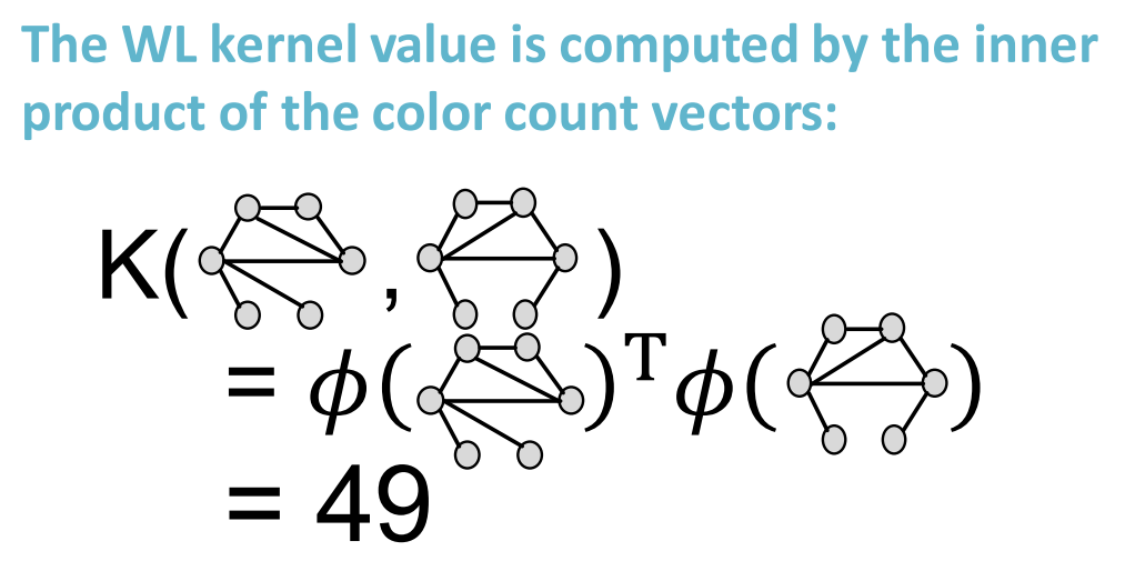
- There exists a feature representation $\phi(\cdot)$ such that $K(G,G’)=\phi(G)^{T}\phi(G’)$
- Once the kernel is defined, off-the-shelf ML model, such as kernel SVM, can be used to make predictions.
- Graph Kernels: Measure similarity between two graphs:
- Graph Kernel
- Weisfeiler-Lehman Kernel
- Other kernels are also proposed in the literature (beyond the scope of this lecture)
- Random-walk kernel
- Shortest-path graph kernel
- And many more …
- Graph kernel key idea
- Bag-of-Words (BoW) for a graph
- Recall: BoW simply uses the word counts as features for documents (no ordering considered)
- Naive extension to a graph: Regard nodes as words.
- Since both graphs have 4 red nodes, we get the same feature vector for two different graphs…
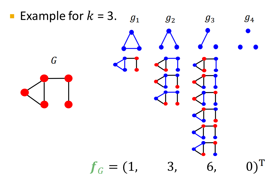
- Graphlet
- Count the number of different graphlets in a graph
- Note: Definition of graphlets here is slightly different from node-level features
- The two differences are:
- Nodes in graphlets here do not need to be connected (allows for isolated nodes)
- The graphlets here are not rooted.
- Examples in the next slide illustrate this.
- Bag-of-Words (BoW) for a graph
- Weisfeiler-Lehman Kernel
- Goal: Design an efficient graph feature descriptor $\phi(G)$
- Idea: Use neighborhood structure to iteratively enrich node vocabulary.
- Generalized version of Bag of node degrees since node degrees are one-hop neighborhood information.
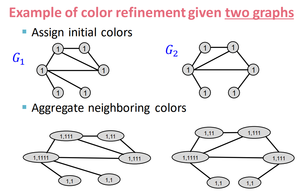
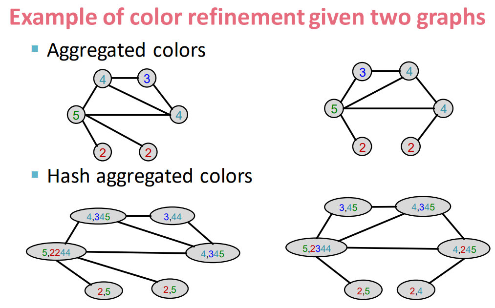
- Color refinement algorithm:
- Given a graph $G$ with a set of nodes $V$.
- Assign an initial color $c^{(0)}(v)$ to each node $v$.
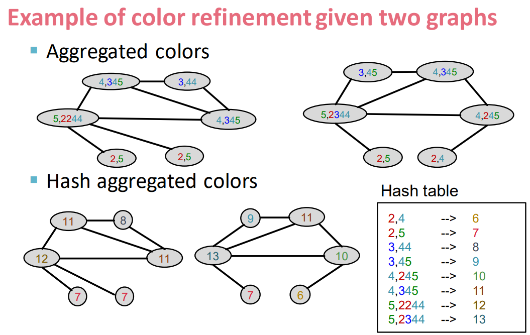
- Iteratively refine node colors by \(c^{(k+1)}(v)=\text{HASH}(\{c^{(k)}(v),\{c^{(k)(u)}\}_{u\in{N(v)}} \})\)
- where $\text{HASH}$ maps different inputs to different colors
- After $K$ steps of color refinement, $c^{(K)}(v)$ summarizes the structure of $K$-hop neighborhood
- Given a graph $G$ with a set of nodes $V$.
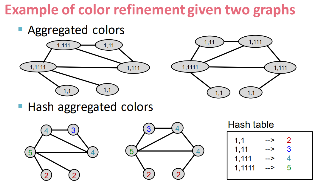
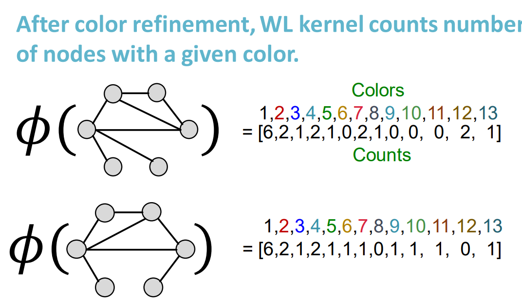
- Weisfeiler-Lehman Kernel
- WL kernel is computationally efficient
- The time complexity for color refinement at each step is linear in #(edges), since it involves aggregating neighboring colors.
- When computing a kernel value, only colors appeared in the two graphs need to be tracked.
- Thus, #(colors) is at most the total number of nodes.
-
Counting colors takes linear-time w.r.t. #(nodes).
- In total, time complexity is linear in #(edges).
- WL kernel is computationally efficient
- Graph-Level Features: Summary
- Graphlet Kernel
- Graph is represented as Bag-of-graphlets
- Computationally expensive
- Weisfeiler-Lehman Kernel
- Apply $K$-step color refinement algorithm to enrich node colors
- Different colors capture different $K$-hop neighborhood structures
- Graph is represented as Bag-of-colors
- Computationally efficient
- Closely related to Graph Neural Network
- Apply $K$-step color refinement algorithm to enrich node colors
- Graphlet Kernel
8. Application of Graph Neural Networks
8.1 Graph Augmentation for GNNs
- General GNN Framework
- Idea: Raw input graph $\neq$ computational graph
- Graph feature augmentation
- Graph structure augmentation
- Idea: Raw input graph $\neq$ computational graph
- Why Augment Graphs
- Our assumption so far has been
- Raw input graph = computational graph
- Reasoning for breaking this assumption
- Features:
- This input graph lacks features
- Graph structure:
- The graph is too sparse -> inefficient message passing
- The graph is too dense -> message passing is too costly
- The graph is too large -> cannot fit the computational graph into a GPU
- Features:
- It is unlikely that the input graph happens to be the optional computation graph for embeddings
- Our assumption so far has been
- Graph Augmentation Approaches
- Graph feature augmentation
- The input graph lacks features -> feature augmentation
- Graph structure augmentation
- The graph is too sparse -> Add virtual nodes / edges
- The graph is too dense -> Sample neighbors when doing message passing
- The graph is too large -> Sample subgraphs to compute embeddings
- Graph feature augmentation
- Add Virtual Nodes / Edges
- Motivation: Augment sparse graphs
- (1) Add virtual edges
- Common approach: Connect 2-hop neighbors via virtual edges
- Intuition: Instead of using adj. matrix $A$ for GNN computation, use $A+A^2$
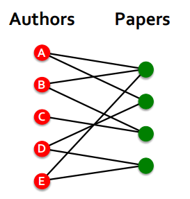
- Use cases: Biparite graphs
- Author-to-papers (they authored)
- 2-hop virtual edges make an author-author collaboration graph
- Add Virtual Nodes / Edges
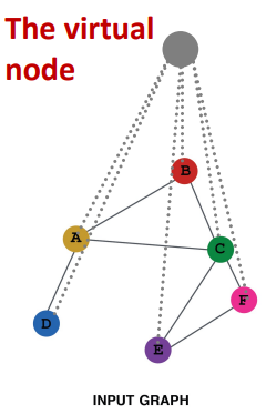
- (2) Add virtual nodes
- The virtual node will connect to all the nodes in the graph
- Suppose in a sparse graph, two nodes have shortest path distance of 1o
- After adding the virtual node, all the nodes will have a distance of two
- Node A - Virtual node - Node B
- Benefits: Greatly improves message passing in sparse graphs
- The virtual node will connect to all the nodes in the graph
- (2) Add virtual nodes
- GNN Training Pipelines
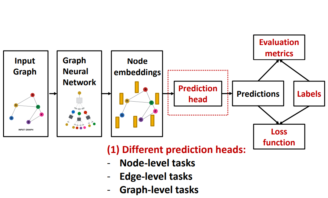
- Prediction Heads: Graph-level
- (1) Global mean pooling
- (2) Global max pooling
- (3) Global sum pooling
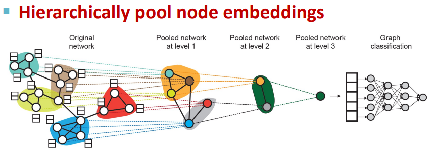
- Issue of Global Pooling
- Issue: Global pooling over a (large) graph will lose information
- Solution: DiffPool
9. Theory of Graph Neural Networks
9.1 How expressive are GNNs?
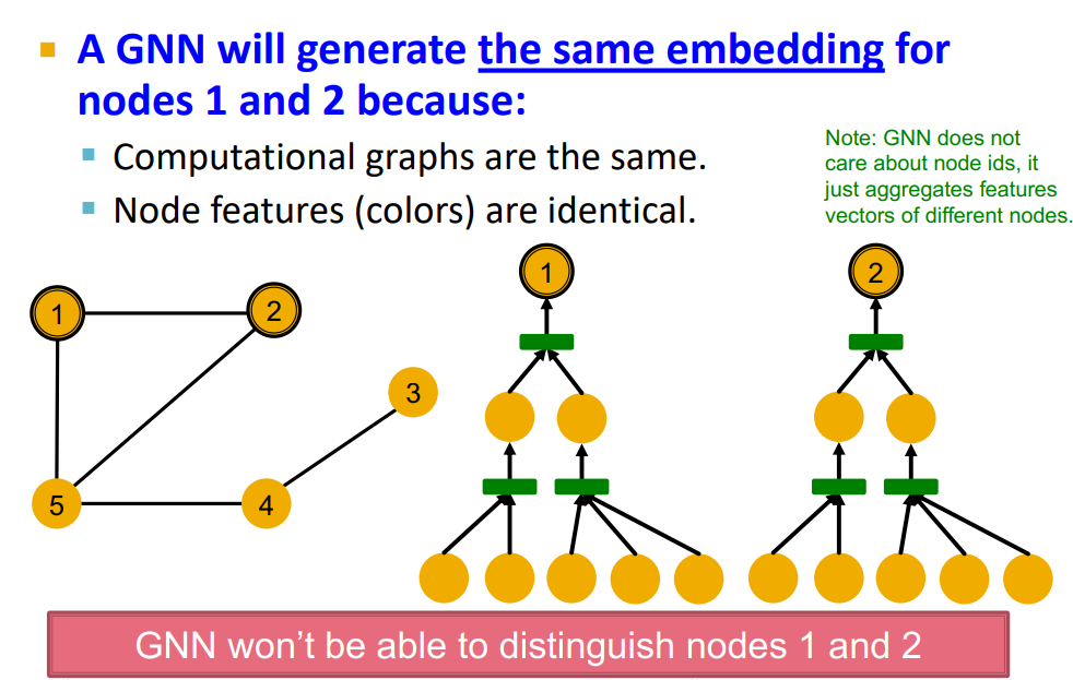
- What is the expressive power (ability to distinguish different graph structures) of these GNN models?
- Ex: GNN won’t be able to distinguish nodes 1 and 2
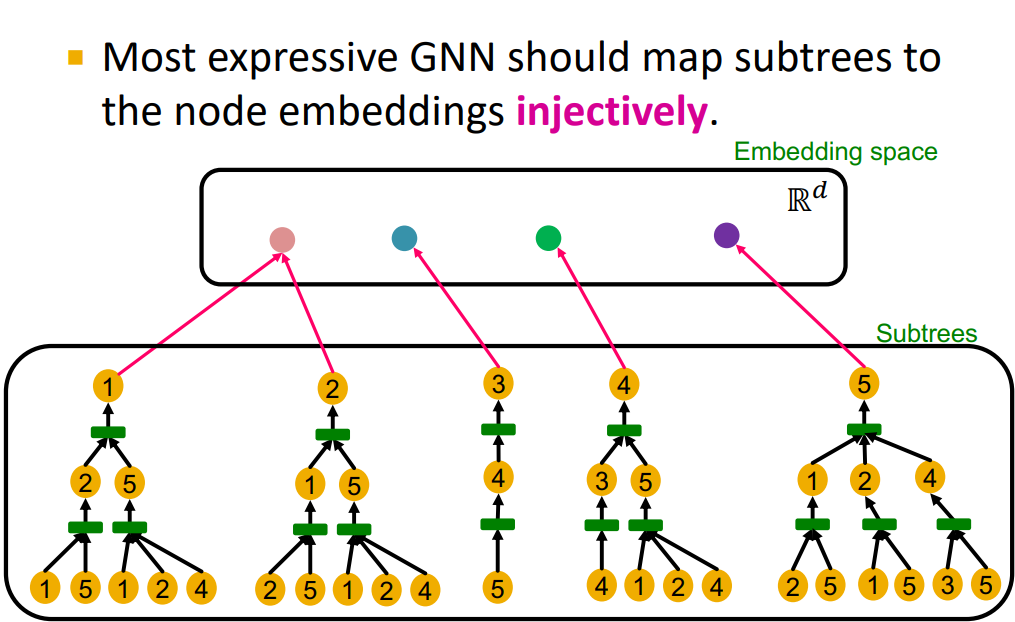
9.2 Design the Most Powerful GNNs
- Our goal: Design maximally powerful GNNs in the class of message-passing GNNs
- This can be achieved by designing injective neighbor aggregation function over multi-sets.
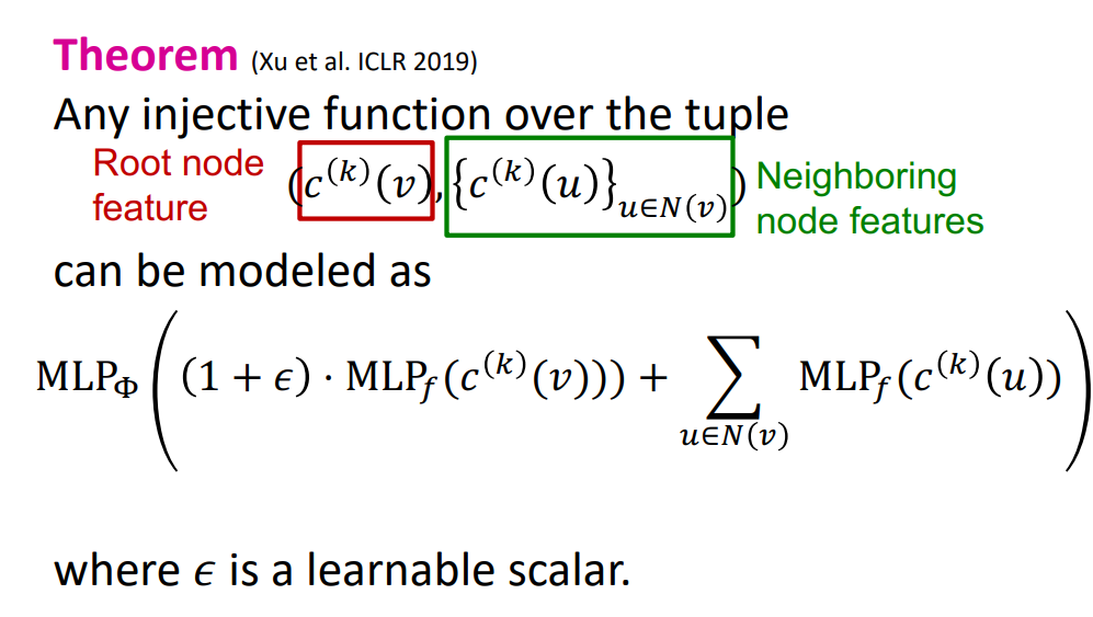
-
Here, we design a neural network that can model injective multiset function.
- Universral Approximation Theorem
- Cited from [Hornik et al., 1989]
- We have arrived at a neural network that can model any injective multiset function
- Graph Isomorphism Network (GIN)
- Apply an MLP, element-wise sum, followed by another MLP
- Full Model of GIN
- We now describe the full model of GIN by relating it to WL graph kernel (traditional way of obtaining graph-level features).
- GIN and WL Graph Kernel
-
GIN can be understood as differentiable neural version of the WL graph Kernel
-
Advantages of GIN over the WL graph kernel are:
- Node embeddings are low-dimensional; hence, they can capture the fine-grained similarity of different nodes.
- Paraemters of the update function can be learned for the downstream tasks.
-
- Expressive Power of GIN
- Because of the relation between GIN and the WL graph kernel, their expressive is exactly the same.
- If two graphs can be distinguished by GIN, they can be also distinguished by the WL kernel, and vice versa.
- Because of the relation between GIN and the WL graph kernel, their expressive is exactly the same.
- Summary of the lecture
- We design a neural network that can model injective multi-set function
- We use the neural network for neighbor aggregration function and arrive at GIN–the most expressive GNN model.
- The key is to use element-wise sum pooling, instead of mean-/max-pooling.
- GIN is closely related to the WL graph kernel.
- Both GIN and WL graph kernel can distinguish most of the real graphs!
10. Heterogenous Graphs and Knowledge Graph Embeddings
10.1 Heterogeneous Graphs and Relational GCN (RGCN)
- Heterogeneous Graphs
- A heterogeneous graph is defined as \(G=(V,E,R,T)\)
- Nodes with node types $v_i\in{V}$
- Edges with relation types $(v_i,r,v_j)\in{E}$
- Node type $T(v_i)$
- Relation type $r\in{R}$
- Example
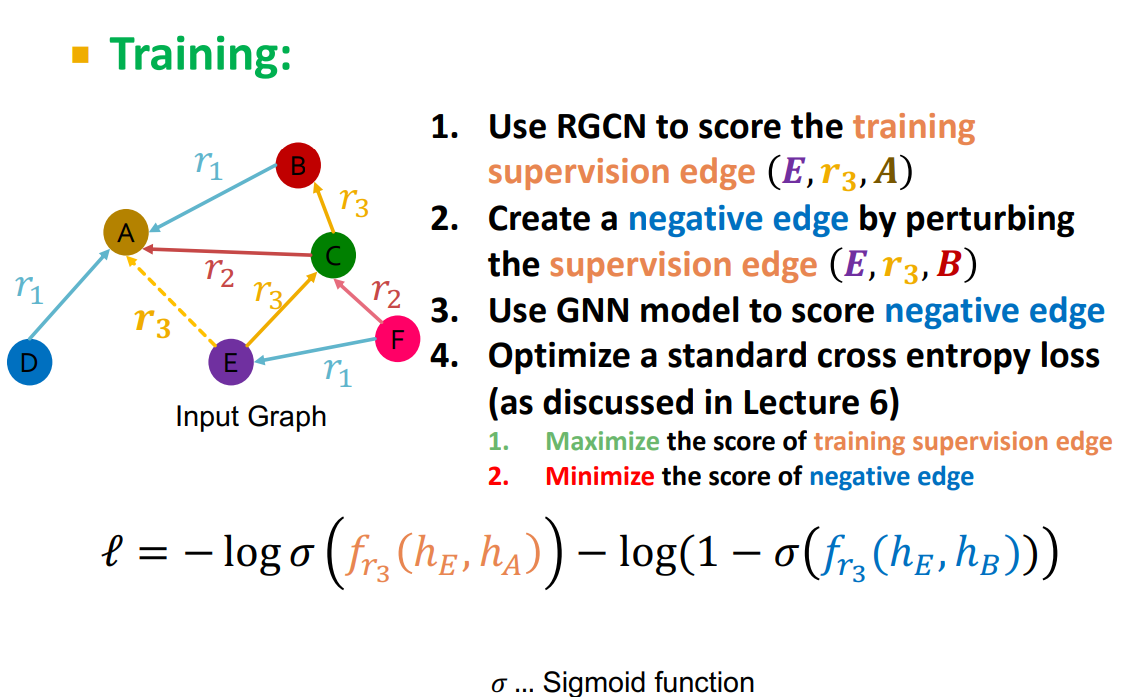
- RGCN for Link Prediction
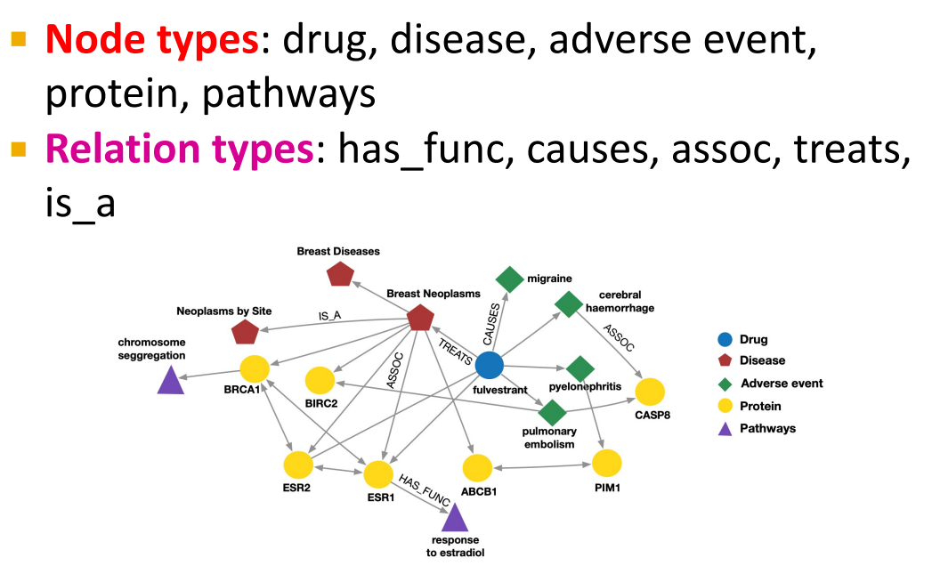
10.2 Knowledge Graphs: KG Completion with Embeddings
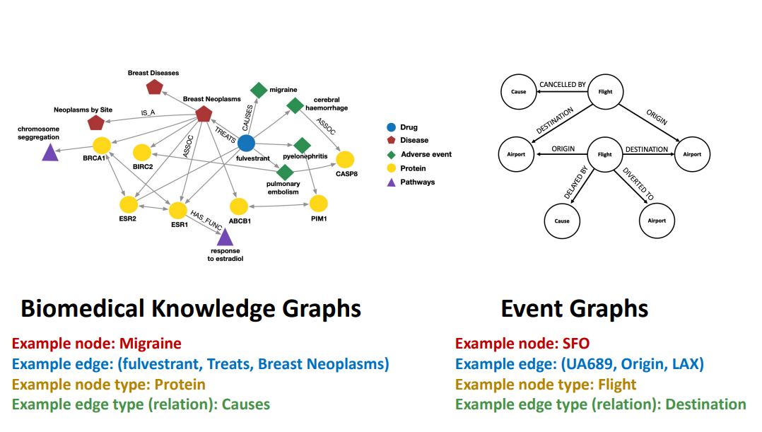
-
Knowledge Graphs (KG) is an example of a heterogeneous graph
-
Example: Bibliographic Networks
10.3 Knowledge Graph Completion: TransE, TransR, DistMul, ComplEx
- KG Representation
- Edges in KG are represented as triples $(h,r,t)$
- head $(h)$ has relation $(r)$ with tail $(t)$
- Key Idea:
- Model entities and relations in the embedding/vector space $\mathbb{R}^{d}$.
- Associtate entities and relations with shallow embeddings
- Note we do not learn a GNN here!
- Given a true triple $(h,r,t)$, the goal is that the embedding of $(h,r)$ should be close to the embedding of $t$.
- How to embed $(h,r)$?
- How to define closeness?
- Model entities and relations in the embedding/vector space $\mathbb{R}^{d}$.
- Edges in KG are represented as triples $(h,r,t)$
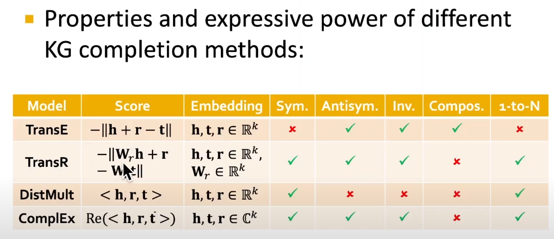
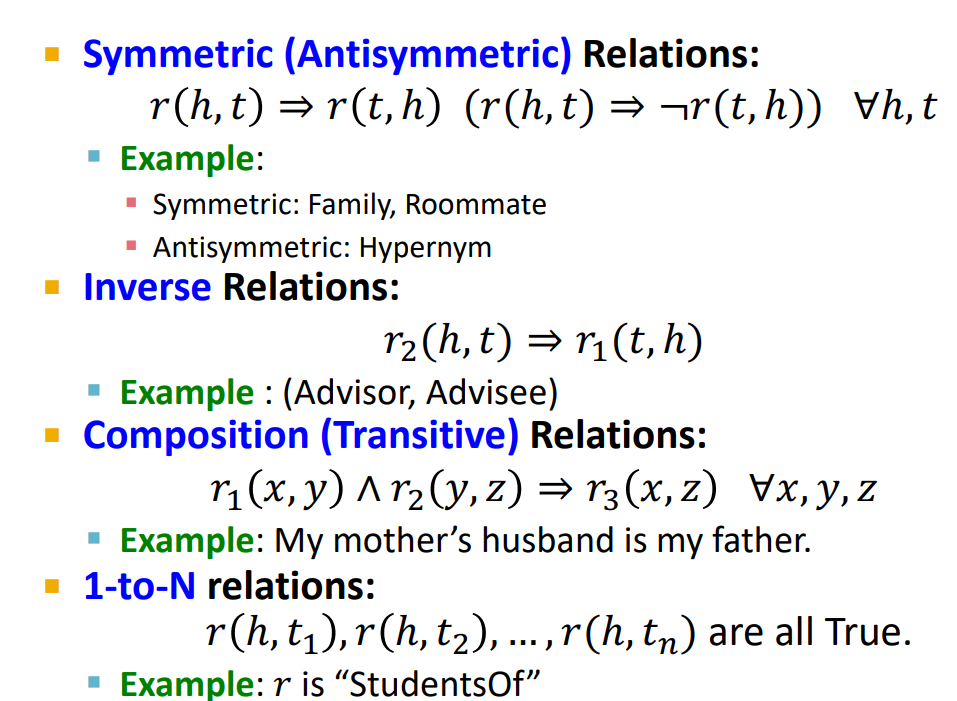
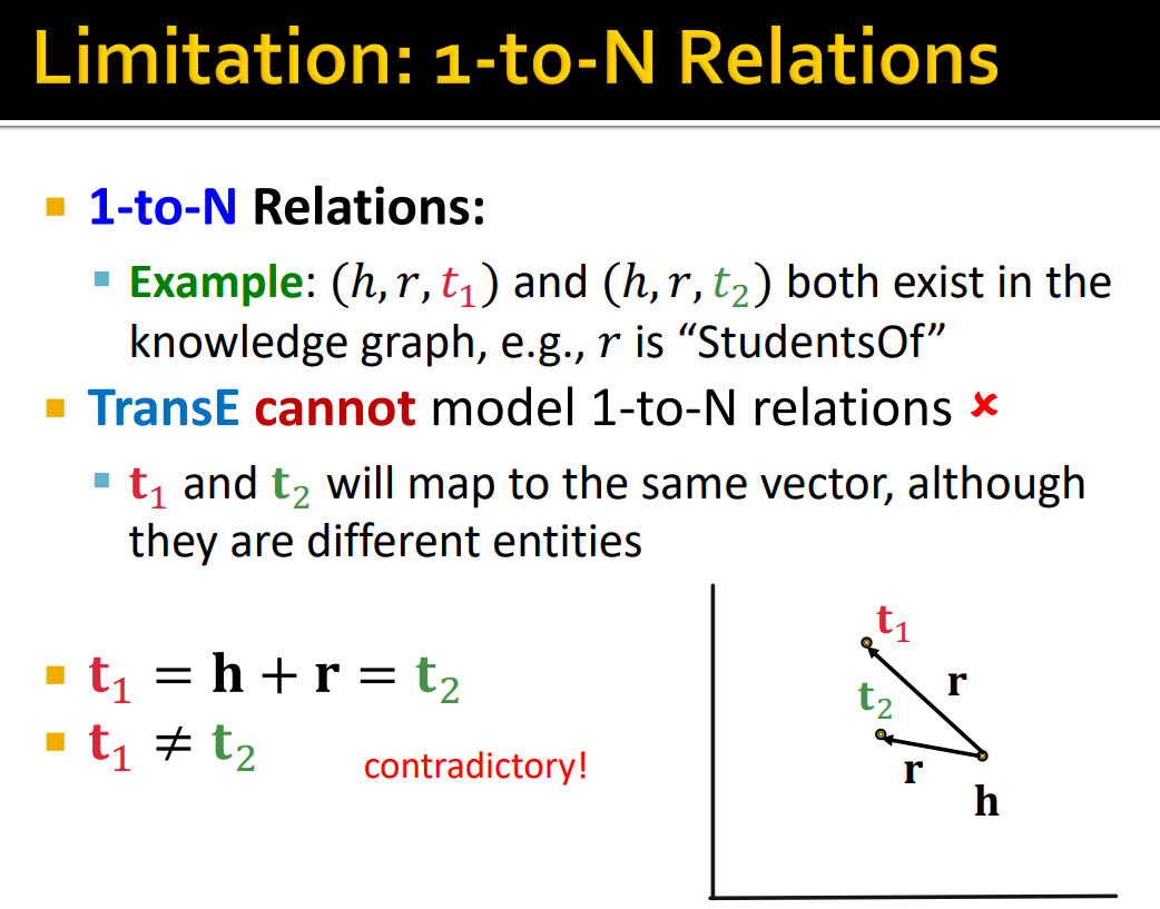
- Relations Patterns
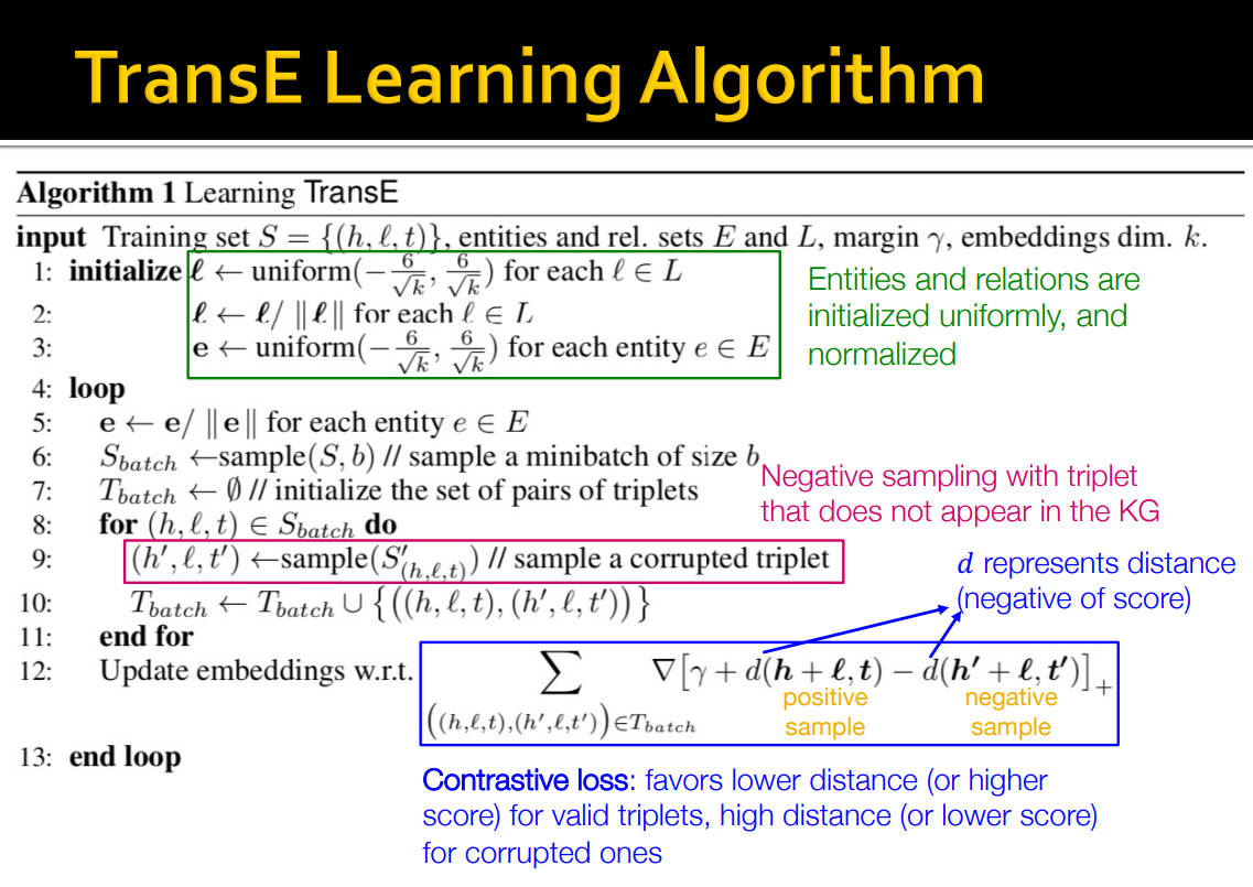
- TransE Learning Algorithm
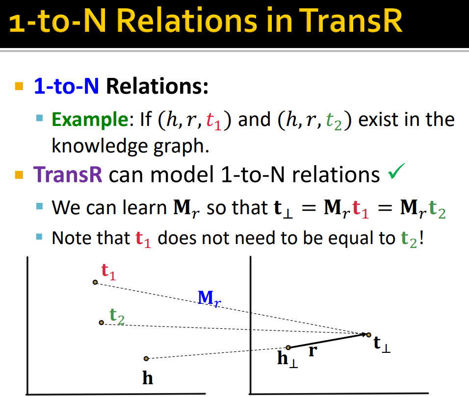
- TransR Learning Algorithm
- DistMult Algorithm
- DistMult: Entities and relations using vectors in $\mathbb{R}^{k}$
- Score function: $f_{r}(h,t)=<\textbf{h,r,t}>=\sum_{i}{\textbf{h}{i}\cdot{\textbf{r}{i}}\cdot{\textbf{t}_{i}}}$
- $\textbf{h,r,t}\in{\mathbb{R}^{k}}$
- Intuition of the score function: Can be viewed as a cosine similarity between $\textbf{h}\cdot{\textbf{r}}$ and $\textbf{t}$
- where $\textbf{h}\cdot{\textbf{r}}$ is defined as $\sum_{i}{\textbf{h}{i}\cdot{\textbf{r}{i}}}$
- Knowledge Graph Completion: ComplEx
- Based on Distmult, ComplEx embeds entities and relations in Complex vector space
- ComplEx: model entities and relations using vectors in $\mathbb{C}^{k}$
- Expresiveness of All Models