Application on Machine Learning

view on github

• 1. Decision Trees
  • 1.1 Entropy
  • 1.2 Information Gain
  • 1.3 Decision Tree/ ID3 Pros and Cons
  • 1.4 Addressing Overfitting
  • 1.5 Pruning Process
• 2. Bagging Trees
  • 2.1 Bagging
    • 2.1.1 Bootstrapping
    • 2.1.2 Aggregating
  • 2.2 Bagging Decision Trees
  • 2.3 Random forests
  • 2.4 Random Forests and Feature Selection
• 3. Boosting
  • 3.1 Decision Stumps
  • 3.2 AdaBoost
  • 3.3 Exponential Loss and Greedy Algorithm
  • 3.4 Out-of-Sample Error
• 4. Nearest Neighbour
  • 4.1 Introduction to Nearest Neighbour
  • 4.2 Generallization of Nearest Neighbour
  • 4.3 k-Nearest Neighbour(kNN)
  • 4.4 Condensed Nearest Neighbour(CNN)
  • 4.5 Parametric vs. Non-parametric
  • 4.6 Radial Basis Functions(RBF)
• 5. Support Vector Machine
  • 5.1 Maximal Margin Linear Separators
  • 5.2 How to calculate the margin?
  • 5.3 Why maximal margin?
  • 5.4 Soft-Margin SVMs
• 6. Neural Networks
  • 6.1 Combining Perceptrons
  • 6.2 Backpropagation
  • 6.3 Regulation
  • 6.4 MLP as Universal Approximators

---

1. Decision Trees

---

1.1 Entropy

Value: the lower a collection’s entropy, the more pure it is

\[Entropy(S)=\sum_{v\in{V(S)}}-\frac{|S_v|}{S}{\log_2}(\frac{|S_v|}{S})\]

1.2 Information Gain

\[IG(x_i,y)= Entropy(y)-\sum_{v\in{V(x_i)}}(f_v)(Entropy(y_{x_i=v}))\]

Where $x_i$ is a feature

• $y$ is the collection of all labels
• $V(x_i)$ is the set of unique values of $x_i$
• $f_v$ is the fraction of inputs where $x_i=v$
• $y_{x_i=v}$ is the collection of labels where $x_i=v$

1.3 Decision Tree/ ID3 Pros and Cons

• Pros:
  • Intuitive and explainable
  • Can handle categorical and real-valued features
  • Automatically performs feature selection
  • The ID3 algorithm has a perference for shorter trees(Simpler hypotheses)
• Cons
  • The ID3 algorithm is a greedy(it selects the feature with highest information gain at every step), so no optimality guarantee.
  • Overfitting! (Achieve zero in sample error)

1.4 Addressing Overfitting

• Heuristics(“regularization”)
  • Do not split leaves past a fixed depth $\delta$
  • Do not split leaves with fewer than $c$ labels
  • Do not split leaves where the maximal information gain is less than $\tau$
  • Predict the most common label at each leaf
• Pruning(“validation”)
  • Evaluate each split using a validation set
  • Compare the validation error with and without that split(replacing it with most common label at that point)

1.5 Pruning Process

Input: a decision tree $t$, and a validation dataset, $\mathcal{D}{val}$
Compute the validation error of tree $t$, and get $E{val}(t)$ For each split $s$ in $t$

• Compute $E_{val}(t\backslash{s})=$ the validation error of $t$ with $s$ replaced by a leaf using the most common label at $s$.
• If exist a split $s\in{t}$, s.t. $E_{val}(t\backslash{s})\leq{E_{val}(t)}$, repeat the pruning process with $t\backslash{s^{}}$, where $t\backslash{s^{}}$ is the pruned tree with minimal validation error.

Double check the pruned tree. If $E_{val}(t)=0$, this means that we cannot prune this tree any more.

2. Bagging Trees

---

2.1 Bagging

Bagging is short for Bootstrap aggregating, which combines the prediction of many hypotheses to reduce variance. If $n$ independent random variables $x_1, x_2,\cdots, x_n$ have variance $\sigma^2$, then the variance of $\frac{1}{n}\sum_{i=1}^{n}{x_i}$ is $\frac{\sigma^2}{n}$

2.1.1 Bootstrapping

Bootstrapping is a statistical method for estimating properties of a distribution, given potentially a small number of samples from that distribution.

Bootstrapping relys on resampling the samples with relacement many, many times:

• Example: {1,2,3,4,5}
• Without replacement {1,1,2,2,3}(Wrong)
• With replacement {1,1,2,2,3}(Allowed)

Bootstrapping Example:

• Suppose you draw 8 samples from a distribution $\mathcal{D}$
• Resample 8 values(with replacement) from $\mathcal{D}$ 1000 times
• Meaning that you will get 1000 sets of 8 values

2.1.2 Aggregating

Aggregating will combine multiple hypotheses. For following types of machine learning tasks, aggregating will:

• Regression: average the predictions;
• Classification: find the category that most hypotheses predict(plurality vote)

2.2 Bagging Decision Trees

Input: $\mathcal{D}, B$ For $b=1,2,\cdots,B$

• Create a dataset, $\mathcal{D}_{b}$, by sampling $n$ points from $\mathcal{D}$ with replacement
• Learn a decision tree, $t_b$, using $D_b$ and the ID3 algorithm Output: $\bar{t}$, the aggregated hypothesis

But the problem is that predictions made by trees trained on similar datasets are highly correlated.

2.3 Random forests

To decorrelate these predictions, we want to use Split-Feature Randomization with randomly limit features avaliable at each iteration of ID3 algorithm. And we will select $m<d$ features every time.

Input: $\mathcal{D}, B, m$

For $b=1,2,\cdots,B$

• Create a dataset, $\mathcal{D}_{b}$, by sampling $n$ points from $\mathcal{D}$ with replacement
• Learn a decision tree, $t_b$, using $D_b$ and the ID3 algorithm with split-feature randomization
  Output: $\bar{t}$, the aggregated hypothesis

2.4 Random Forests and Feature Selection

Random forests allow for the computation of “variable importance”, a way of ranking features based on how useful they are at predicting the output.

• Initialize each feature’s importance to zero
• Each time a feature is chosen by the ID3 algorithm(with split-feature randomization), add that feature’s information gain(relative to the split) to its importance.

3. Boosting

---

Another Cons for Decision Tree is High Bias(Especially short trees, i.e. stumps). Therefore, we introduce a new way - Boosting.

3.1 Decision Stumps

• Weak learner
• Tend to use with boosting
• Assemble them to make up a much better learner(complex one)

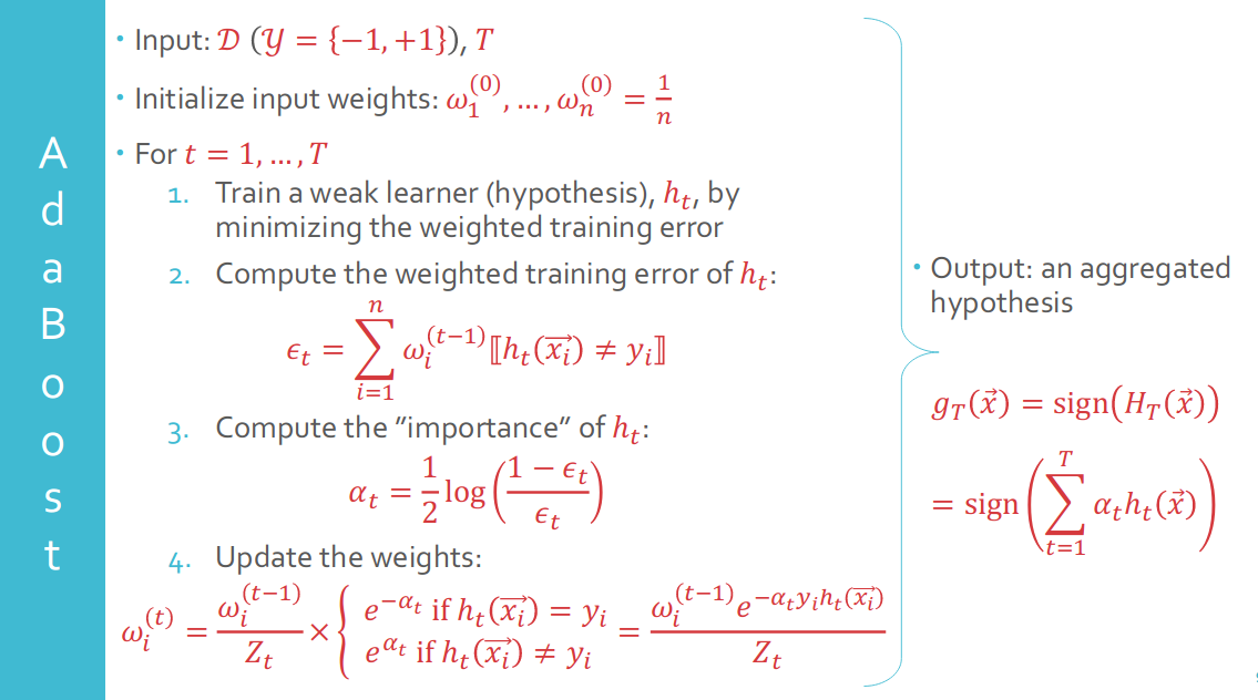
3.2 AdaBoost

Why AdaBoost?

• Only have access to weak learner(Computational Restraints)
• Want final hypothesis to be a weighted combination of weak learners
• Greedily minimize exponential loss(upper bounds for binary error)

• Setting $\alpha_t$: Intuitively, we want good hypotheses to have high weights.

• Normalizring $w_i$: Trying to use sum of each points’ weights $\omega_i$ to normalize updated weights

Exponential Loss

• $e^{-f({\mathbf{x}})h(\mathbf{x})}$
• Used for binary classification, and the more $h(\mathbf{x})$ agrees with $f(\mathbf{x})$, the smaller the loss.
• Also, we can claim that:

\[e^{-f({\mathbf{x}})h(\mathbf{x})}\leq{[|f({\mathbf{x}})\neq{h(\mathbf{x})}|]}\]

3.3 Exponential Loss and Greedy Algorithm

Final Exponentail Loss

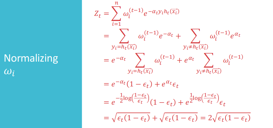
\[\frac{1}{n}\sum_{i=1}^{n}{ e^{-y({\mathbf{x}_i})H_{T}({\mathbf{x}_i}) }}= \prod_{t=1}^{T}{Z_{t}}\]

Then, if we want to achieve the mimimal loss at the final loss, we want to make each $Z_t$ is minimal at each iteration with greedy algorithm.

Then, we are going to prove that choosing $\alpha_t=\frac{1}{2}{ \log{ \frac{(1-{\epsilon}_t)}{\epsilon_t}}}$ will be good with regard to greedy algorithm.

Therefore, the in-sample error will finally be very small, since($Z_t<1$):

\[\prod_{t=1}^{T}{Z_t}=\prod_{t=1}^{T}{2\sqrt{\epsilon_t(1-\epsilon_t)}}\rightarrow0\]

3.4 Out-of-Sample Error

Emprical Results indicate that increasing T does not lead to overfitting as this bound would suggest.

Margins: can be interpreted as how confident $g_T$ is in its prediction: the bigger the margin, the more confident.

Tips: $n$ increase, I think that the model will become more inconfident.

4. Nearest Neighbour

---

4.1 Introduction to Nearest Neighbour

• Euclidean Distance
• Cosine similarity
• Mahalanobis Distance

Nearest Neighbour:
Let $\mathbf{x}_{[1]}{\mathbf{x}}$ be $\mathbf{x}$’s nearest neighbour, i.e. the closest point to $\mathbf{x}$ in $\mathcal{D}$
The nearest neighbour hypothesis

• $g(\mathbf{x})=y_{[1]}(\mathbf{x})$
• Require no training!
• Always no training error!(Can always shatter points)

4.2 Generallization of Nearest Neighbour

Claim: $E_{out}$ for the nearest neighbour hypothesis is not much worse than the best possible $E_{out}$

Formally: under certain conditions, with high probability, $E_{out}(g)\leq{2{E}_{out}(g^{*})}$ as $n\rightarrow{\infty}$

Proof:

Before proof, here are the assumptions:
(1)Assume a binary classification problem: $\mathcal{Y}={-1,+1}$
(2)Assume labels are noisy:

\[\pi(\mathbf{x})=P\{y=+1|\mathbf{x}\}\]

(3) Assume $\pi(\mathbf{x})$ is continuous
(4) As $n\rightarrow{\infty}$, $\mathbf{x}_{[1]}{\mathbf{x}}\rightarrow{\mathbf{x}}$

Therefore,

\[\begin{aligned} E_{out} & =\mathbb{E}_{\mathbf{x}}\big[[{g(\mathbf{x})\neq{y}}]\big]\\ & =P\{ g(\mathbf{x})=+1 \cap {y=-1}\} + P\{ g(\mathbf{x})=-1 \cap {y=+1}\} \\ & =\pi{(\mathbf{x}_{[1]}{\mathbf{x}})}(1-\pi{(\mathbf{x})}) + \big(1-\pi{(\mathbf{x}_{[1]}{\mathbf{x}})}\big)(\pi{(\mathbf{x})})\\ & = 2\pi(\mathbf{x})(1-\pi(\mathbf{x}))\\ & \leq{2min(\pi(\mathbf{x}),(1-\pi({\mathbf{x}})))}=2E_{out}(g^{*}) \end{aligned}\]

Self-Regularization: The nearest neighbour hypothesis can only be complex when there is more data.

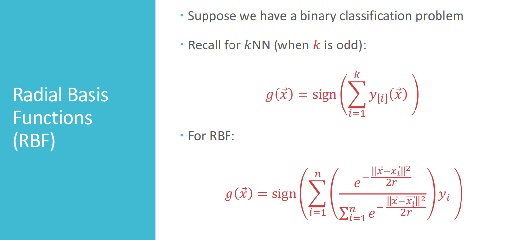
4.3 k-Nearest Neighbour(kNN)

Classify a point as the most common label among the labels of the $k$ nearest training points

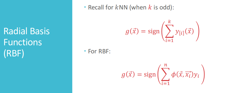
If we have a binary classification probelm and $k$ is odd:

\[g(\mathbf{x})=sign(\sum_{i=1}^{k}{y_{[i]}(\mathbf{x})})\]

Setting $k$

kNN Pros and Cons
For pros, it is (1)Intuitive/explainable; (2)Has No training/retraining; (3)Provably near-optimal in terms of $E_{out}$

As to cons, it is Computationally expensive, which always needs to store all data, and computing $g(\mathbf{x})$ requires computing distances and sorting

4.4 Condensed Nearest Neighbour(CNN)

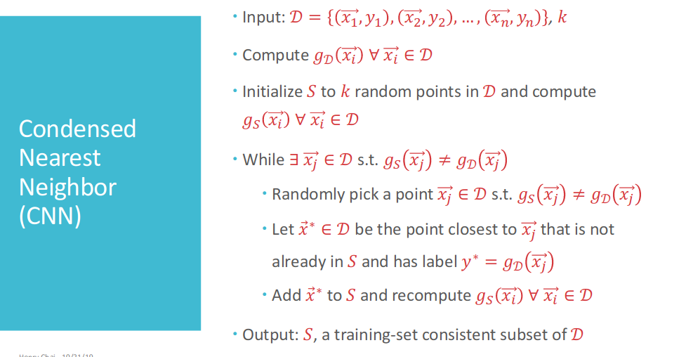
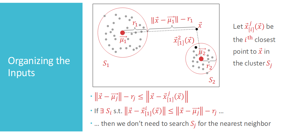
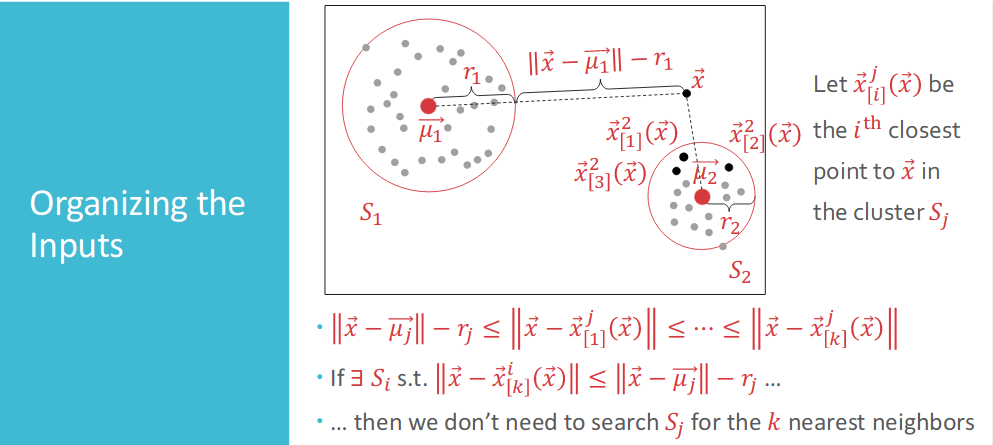
Procedure #1: Organizing the inputs

• Just split the inputs into clusters, groups of points that are close to one another but far from other groups.

• The figure above shows us that if we have a point in set $i$, and the distance between $\mathbf{x}$ and it is less than $\mathbf{x}$ to set $j$’s boundary, then we do not need to search points in set $j$ any more.

• Further more, we promote this therom to wider application

Procedure #2: Clustering inputs

• Using Triangle Inequality in norm, we have

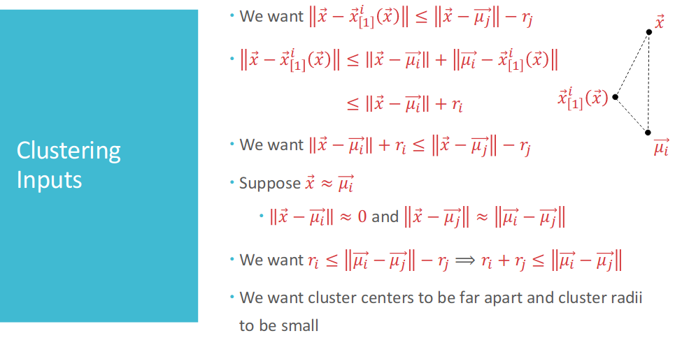
• Therefore, we want cluster centers to be far apart and cluster radii to be small

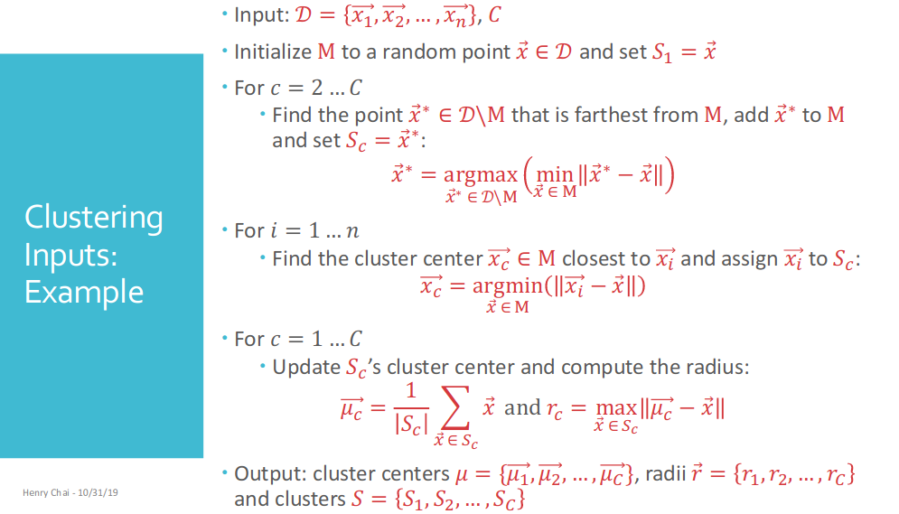
• Explanation about pitcture above:
  • 1st Step is about how to generate center points in each cluster;
  • 2nd Step is about how to assign every points in data set $\mathcal{D}$ to $C$ clusters
  • 3rd Step is about after assigned point to each cluster, we need to update its center point and the radius

4.5 Parametric vs. Non-parametric

Parametric Model

• Hypotheses have a parametrized form
• Parameters learned from training data; can discard training data afterwards;
• Cannot exactly model every target function

Non Parametric Models

• Hypotheses cannot be expressed using a finite number of parameters
  • Example: kNN, decision trees
• Training data generally need to be stored in order to make predictions
• Can recover any target function given enough data

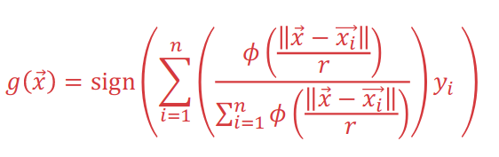
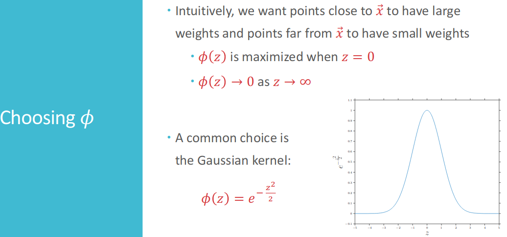
4.6 Radial Basis Functions(RBF)

• kNN only consider some points and weights them equally
• What if we considered all points but weighted them unequally?
• Intution: all points are useful but some points are more useful than others!
• Bouns: no need to choose $k$

Suppose we have a binary classification problem

• If $r$ is really small, then $\frac{|\mathbf{x}-\mathbf{x}_i|}{r}$ will always be large (unless $|\mathbf{x}-\mathbf{x}_i|$ is small)
• If $\frac{|\mathbf{x}-\mathbf{x}_i|}{r}$ is large, then $\phi(\frac{|\mathbf{x}-\mathbf{x}_i|}{r})$ will always be small(unless $|\mathbf{x}-\mathbf{x}_i|$ is small)
• The smaller $r$ is, the closer $\mathbf{x}$ has to be to $\mathbf{x}_i$ in order for $\phi(\frac{|\mathbf{x}-\mathbf{x}_i|}{r})$ to be non-zero

In a sense, $r$ is like $k$, if $r$ increases, we care more and more points.

Intutively, we want points close to $\mathbf{x}$ to have larger weights and points far from $\mathbf{x}$ to have small weights

And finally, we have

5. Support Vector Machine

---

5.1 Maximal Margin Linear Separators

We want maximum the margin with restraint on correct classification.

\[\begin{aligned} &\textbf{max}\ margin(\mathbf{w})\\ &\textbf{subject\ to\ } \mathbf{w}\ classify\ every\ (\mathbf{x}_i,y_i)\ correctly \end{aligned}\]

We can use special scaling and make every linear separators become separating hyperplanes.

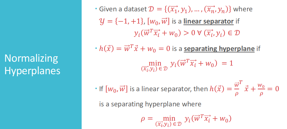
After scaling our weight vector, every separating hyperplane have margin expression:

\[\frac{1}{\|\mathbf{w}\|}\]

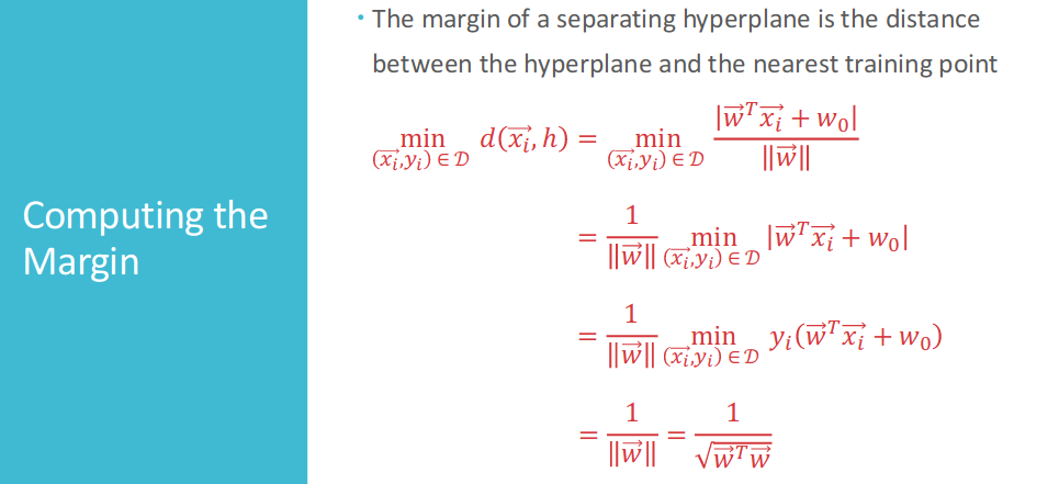
5.2 How to calculate the margin?

First, we want to prove that weight vector $\mathbf{w}$ is orthogonal to the hyperplane $h(\mathbf{x})=\mathbf{w^{T}x}+w_0=0$

Second, we will use the knowledge of projection. Suppose $\mathbf{x}’$ be an arbitrary point on the hyperplane, and $\mathbf{x}’’$ be an arbitrary point. The distance between $\mathbf{x}’’$ to the hyperplane $h(\mathbf{x})=\mathbf{w^{T}x}+w_0=0$ will be

\[d(x'', h)=|\frac{\mathbf{w^{T}(\mathbf{x''}-\mathbf{x'})}}{\|\mathbf{w}\|}|=|\frac{\mathbf{w^T{x''}}+w_0}{\|\mathbf{w}\|}|\]

The margin of separating hyperplane is the distance between the hyperplane and the nearest training point

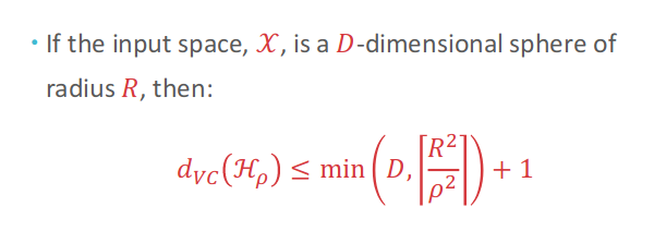
5.3 Why maximal margin?

With minimum margin $\rho$, linear separators in $\mathcal{H}_{\rho}$ can not always shatter all sets of three points.

5.4 Soft-Margin SVMs

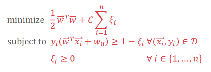
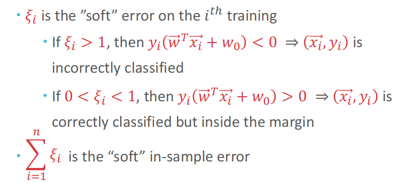
$\xi_i$ is the soft error on the $i^{th}$ training

6. Neural Networks

---

6.1 Combining Perceptrons

A simple and direct idea of Neural Networks is to combine perceptrons to approach the target function.

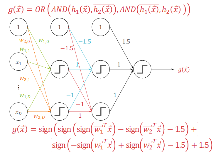
Following is a figure of Multi-Layer Perceptrion (MLP).

The architecture of an MLP is the vector $\vec{d}=[d^{(0)}, d^{(1)},\cdots, d^{(L)}]$.
And the weights between layer $l-1$ and layer $l$ are a matrix: $W^{(l)} \in {\mathbb{R}^{(d^{(l-1)}+1)\times{d^{(l)}}}}$.

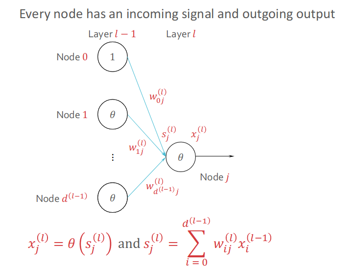
To make clear the Signal and Output for MLP, following figure will demonstrate how each node contributes to the node of next layer.

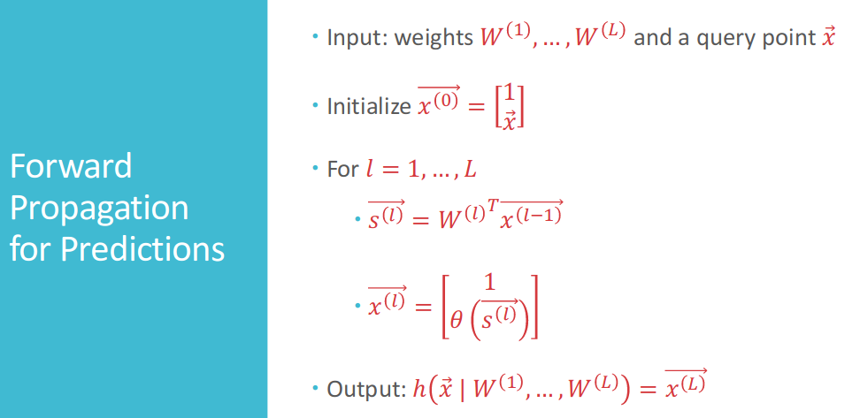
Then we can make Forward Propagation for Predictions:

6.2 Backpropagation

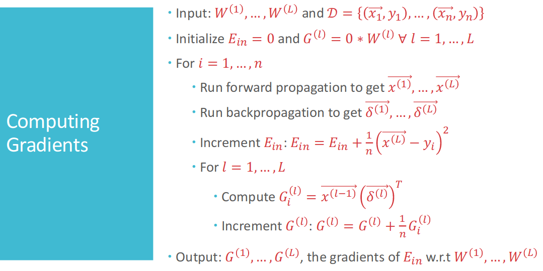
The most important and interesting part of neural network is about backpropagation. To minimize the error function of the huge neural network with forward propagation of predictinos, we need to Compute Gradients:

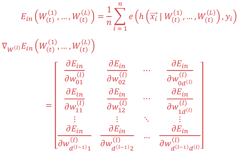
Then we need to Computing Partial Derivatives With Chain Rule:

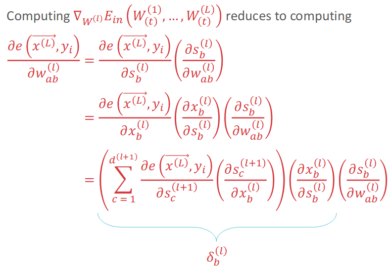
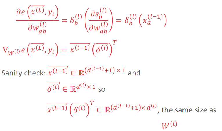
At last, we can check the following for details of whole process of Back Propagation:

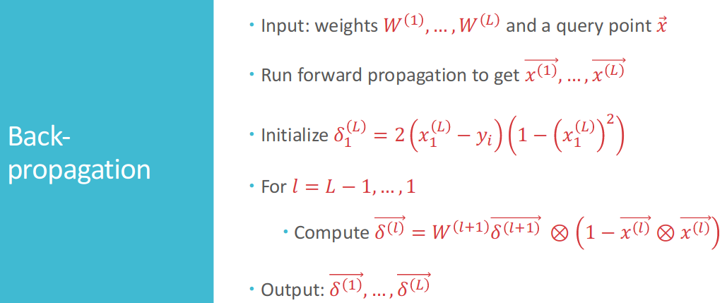
In summary, we will use following figures to describe the Gradients Descent with Feed Forward and Back Propagation:

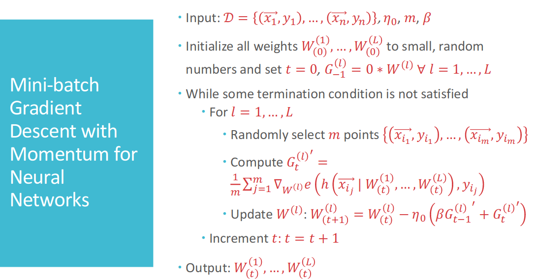
Calculating gradient for full points will cause a huge amount of time. Therefore, we will use Mini-batch Gradient Descent:

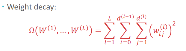
6.3 Regulation

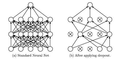
Also, in neural network research, overfitting is a annoying problem. To solve this, we propose to use Regulation:

Also, Dropout Regulation is an effective way:

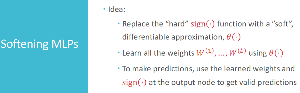
6.4 MLP as Universal Approximators

Therom: Any function that can be decomposed into perceptrons can be modelled exactly using a 3-layer MLP. Any smooth decision boundary can be approximated to an arbitrary precision using a finite number of perceptrons.

Therom: Any smooth decision boundary can be approximated to an arbitrary precision using a 3-layer MLP