Bayesian Machine Learning
view on github- 1. Bayesian Inference
- 2. Bayesian Approach to Regression
Courses Website
1. Bayesian Inference
1.1 Introduction to the Bayesian Method
The goal of probabilistic inference is to make some statements about $\theta$ given these observations.
The Rule of Total Probability
\[Pr(X)=\sum_{i=1}^{N}Pr(X,Y_i)\] \[p(x)=\int_{Y}p(x,y)dy\]Product Rule
\[Pr(X,Y)=Pr(Y|X)Pr(X)\]Bayesian Theorem
\[Pr(Y|X)=\frac{Pr(X|Y)Pr(Y)}{Pr(X)}=\frac{Pr(X|Y)Pr(Y)}{\sum{Pr(X|Y)Pr(Y)}}\]Posterior: $Pr(\theta|D)$
Prior: $Pr(\theta)$
Likelihood: $Pr(D|\theta)$
1.2 Coin Flipping
Suppose that we flip the coin $n$ times and observe $x$ “heads”. Therefore, the probability of this observation, given the value of $\theta$, comes from a binomial distribution:
\[Pr(D|\theta)=Bin(x|n,\theta)=\binom{n}{x}\theta^x(1-\theta)^{n-x}\]Maximum Likelihood
\[\begin{aligned} \hat{\theta}_{MLE} &=\arg{\max_{\theta}}{\ Pr(\mathcal{D}|\theta)}\\ &=\arg{\max_{\theta}}{\text{ Bin}(x|n,\theta)}\\ &=\arg{\max_{\theta}}{\ \binom{n}{x}\theta^{x}{(1-\theta)^{n-x}}}\\ &=\arg{\max_{\theta}}{\ x\text{log}{\theta}+(n-x)\text{log}{(1-\theta)}}\\ &=\frac{x}{n} \end{aligned}\]Maximum A Posterior Emstimation
Since we have formula
\[Pr(\theta|\mathcal{D})=\frac{Pr(\mathcal{D}|\theta)Pr(\theta)}{Pr(\mathcal{D})}\]For a fixed set of observations,
\[Pr(\theta|\mathcal{D}) \propto Pr(\mathcal{D}|\theta)\times{Pr(\theta)}\] \[\color{orangered}{\text{Posterior }} \color{b}{\propto} \color{lightgreen}{\text{ Likelihood }}\color{b}{\times}\color{dodgerblue}{{\text{ Prior }}}\]If $\theta$ is a continuous r.v. with $\color{dodgerblue}{\text{prior p.d.f.}}$ with $\color{dodgerblue}{g(\theta)}$, then its $\color{orangered}{\text{posterior p.d.f.}}$ with $\color{orangered}{f(\theta|\mathcal{D})}$ is given by
\[\color{orangered}{f(\theta|\mathcal{D})}=\color{b}{\frac{\color{lightgreen}{Pr(\mathcal{D}|\theta)}\color{b}{\times}\color{dodgerblue}{g(\theta)}}{Pr(\mathcal{D})}}\]Here, for MAP, since we decide likelihood function with binomial, we can choose beta distribution as prior (details told in Conjugate Priors). Therefore, we have following induction:
\[\begin{aligned} \hat\theta_{MAP} & =\arg{\max_{\theta}}{\ Pr(\theta|\mathcal{D})}\\ & =\arg{\max_{\theta}}{\ Pr(\mathcal{D}|\theta)\cdot{Pr(\theta)}}\\ & =\arg{\max_{\theta}}{\ \theta^{x+\alpha-1}(1-\theta)^{n-x+\beta-1}}\\ & =\frac{x+\alpha-1}{n+\alpha+\beta-2} \end{aligned}\]Conjugate Priors
If the posteriors and priors have the same function form, we call those priors $\color{dodgerblue}{\textbf{conjugate priors}}$. The most famous prior is $\color{dodgerblue}{\textbf{beta distributions}}$, which is a convenient prior for binonmial likelihood and has two parameters $\alpha$ and $\beta$:
\[\begin{aligned} \color{dodgerblue}{g(\theta)=\mathcal{B}(\theta|\alpha,\beta)}\color{b}{=\frac{1}{\color{violet}{\text{Beta}(\alpha,\beta)}}{\theta^{\alpha-1}(1-\theta)^{\beta-1}}} \end{aligned}\]Here, the normalizing constant $\color{violet}{\text{Beta}(\alpha,\beta)}$ is the $\color{violet}{\textbf{beta function}}$.
\[\color{violet}{\text{Beta}(\alpha,\beta)=\int_{0}^{1}{\theta^{\alpha-1}(1-\theta)^{\beta-1}}{d{\theta}}=\frac{\Gamma(\alpha)\Gamma(\beta)}{\Gamma(\alpha+\beta)}}\]Above equation is to ensure that integral of $\color{dodgerblue}{g(\theta)\text{ or }\mathcal{B}(\theta|\alpha,\beta)}$ is one.
General Cases for Posterior of Binomial Distribution
Given our observations $D=(x,n)$, we can now compute the posterior distribution of $\theta$:
\[\color{orangered}{f(\theta|x,n,\alpha,\beta)} \color{b}{=\frac{\color{lightgreen}{Pr(x|n,\theta)}\color{b}{\times}\color{dodgerblue}{g(\theta|\alpha,\beta)}} {\color{violet}{\int{Pr(x|n,\theta)g(\theta|\alpha,\beta)}d{\theta}}}}\]First, we can handle the normalization constant $\color{violet}{Pr(x|n,\alpha,\beta)}$:
\[\begin{aligned} {\color{violet}{\int{Pr(x|n,\theta)g(\theta|\alpha,\beta)}d{\theta}}} &= {\int_{0}^{1}{\binom{n}{x}{\theta}^{x}{(1-\theta)}^{n-x}} \color{b}{\times\frac{1}{\text{Beta}(\alpha,\beta)}}{\theta^{\alpha-1}(1-\theta)^{\beta-1}}d{\theta}}\\ &= \frac{\binom{n}{x}}{\text{Beta}(\alpha,\beta)}\times{\int_{0}^{1}{\theta^{x+\alpha-1}(1-\theta)^{n-x+\beta-1}}d{\theta}}\\ &= \frac{\binom{n}{x}}{\text{Beta}(\alpha,\beta)}\times{\text{Beta}(x+\alpha,n-x+\beta)} \end{aligned}\]Second, we can expand and simplify numerator with:
\[\begin{aligned} \color{lightgreen}{Pr(x|n,\theta)}\color{b}{\times}\color{dodgerblue}{g(\theta|\alpha,\beta)} &= \color{lightgreen}{\binom{n}{x}{\theta^{x}}{(1-\theta)^{n-x}}} \color{b}{\times} \color{dodgerblue} {\frac{1}{\text{Beta}(\alpha,\beta)}{\theta^{\alpha-1}(1-\theta)^{\beta-1}}}\\ &= \frac{\binom{n}{x}}{\text{Beta}(\alpha,\beta)}\times{\theta^{x+\alpha-1}(1-\theta)^{n-x+\beta-1}} \end{aligned}\]Hence, $\color{orangered}{f(\theta|x,n,\alpha,\beta)}$ have:
\[\begin{aligned} \color{orangered}{f(\theta|x,n,\alpha,\beta)} &= \color{b}{\frac{\color{lightgreen}{Pr(x|n,\theta)}\color{b}{\times}\color{dodgerblue}{g(\theta|\alpha,\beta)}} {\color{violet}{\int{Pr(x|n,\theta)g(\theta|\alpha,\beta)}d{\theta}}}}\\ & = \frac{\frac{\binom{n}{x}}{\text{Beta}(\alpha,\beta)}\times{\theta^{x+\alpha-1}(1-\theta)^{n-x+\beta-1}}} {\frac{\binom{n}{x}}{\text{Beta}(\alpha,\beta)}\times{\text{Beta}(x+\alpha,n-x+\beta)}}\\ &= \frac{1} {\text{Beta}(x+\alpha,n-x+\beta)}\times{\theta^{x+\alpha-1}(1-\theta)^{n-x+\beta-1}}\\ &= \mathcal{B}(x+\alpha, n-x+\beta) \end{aligned}\]The posterior $\color{orangered}{f(\theta|x,n,\alpha,\beta)}$ is therefore another beta distribution with parameters $(x+\alpha,n-x+\beta)$.
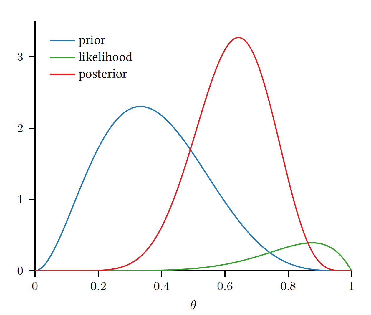
And we find out posterior is still beta distribution with different parameters. The interpreatation of parameters are usually considered as pseudocount.
Their plot are like the following picture:
Special Case for Prior
- Suppose prior representing an expectation of coins biased toward more heads:
- Using above prior, the posterior p.d.f. $f$ is given by:
- From above formula, we will observe one more head than former belief, which is counted with Pseudocount
Posterior Predictive Distributions
With posterior function $\color{orangered}{\textbf{(conjugate priors)}}$ of $\color{orangered}{f(\theta|\mathcal{D})}$ on parameters $\theta$ given observations $\mathcal{D}$, we can compute a distribution on future observations that does not depend on assuming any particular parameter values.
\[Pr(X=x|\mathcal{D})=\int_{-\infty}^{{+\infty}}Pr(X=x|\theta)\color{orangered}{\ f{(\theta|\mathcal{D})}}\color{b}d\theta\]For example:
- When the prior on $\theta$ is $\text{beta}(\alpha,\beta)$, $X$ is a binary random variable with $Pr(X=1)=\theta$.
- Here, $n$ Bernoulli experiments have been observed in which $X=1$ occured $x$ times, above equation becomes:
Here, we re-introduce $\color{violet}{\textbf{beta function}}$ concept.
\[\begin{aligned} \color{violet}{\textbf{beta function}} &:\color{b}{\text{Beta}(\alpha,\beta)=\int_{0}^{1}{\theta^{\alpha-1}(1-\theta)^{\beta-1}}{d{\theta}}=\frac{\Gamma(\alpha)\Gamma(\beta)}{\Gamma(\alpha+\beta)}}\\ \color{violet}{\textbf{beta distribution}} &:\color{b}{\mathcal{B}(\theta|\alpha,\beta)=\frac{1}{\text{Beta}(\alpha,\beta)}{\theta^{\alpha-1}(1-\theta)^{\beta-1}}} \end{aligned}\]Multinomial Distribution
- Here, binomial distribution becomes multinomial distribution.
- Beta distribution becomes Dirichlet prior.
Likelihood
\[Pr(X|\theta)=\text{Mu}(x|\theta)=\prod_{j=1}^{K}{\theta_{j}^{I(x=j)}}\] \[Pr(x|\theta)=\text{Mu}(x|\theta)=\prod_{j=1}^{K}{\theta_{j}^{x_j}}\] \[\begin{aligned} Pr(\mathcal{D}|\theta) &=\prod_{n=1}^{N}\prod_{j=1}^{K}{\theta_{j}^{I(x_{n}=j)}}\ \ \ (D=\{x_1,x_2,\cdots,x_N \})\\ Pr(N_1,N_2,\cdots,N_k|N) &=\text{Mu}(\theta,N)=\binom{N}{N_1,N_2,\cdots,N_k}\prod_{j=1}^{K}{\theta_{j}^{N_j}} \end{aligned}\]For example,
\[Pr(x_1,x_2,x_3|\theta_1,\theta_2,\theta_3)=\frac{(x_1+x_2+x_3)!}{x_1!x_2!x_3!}{\ \theta_1^{x_1}}{\theta_2^{x_2}}{\theta_3^{x_3}}\]1.3 Hypothesis Testing and Summarizing Distributions
To measure a problem like is this coin fair? or Does $\theta=\frac{1}{2}$ ?, we have following approaches from perspective of Bayesian or Frequentist.
Hypothesis Testing - Bayesian
We first derive the posterior distribution $p(\theta|\mathcal{D})$ and then may conpute the probability of the hypothesis directly:
\[Pr(\theta\in\mathcal{H}|\mathcal{D})=\int_{\mathcal{H}}{p(\theta|\mathcal{D})}d{\theta}\]For example, we are interested in the unknown bias of a coin $\theta\in{(0,1)}$, and begin with the uniform prior on the interval $(0,1)$:
\[p(\theta)=\mathcal{U}(\theta;0,1)=\mathcal{B}(\theta;\alpha=1,\beta=1)\]Then, let’s collect some data to further inform our belief about $\theta$. Suppose we flip the coin independently $n=50$ times and observe $x=30$ heads. After gathering this data, we wish to consider the natural question of is this coin fair? or Does $\theta=\frac{1}{2}$ ?
From above experiment, we can compute the posterior distribution easily. It is an updated beta distribution:
\[p(\theta|\mathcal{D})=\mathcal{B}(\theta;31,21)\]Therefore, we may now computer the posterior probability of the hypothesis that the coin is fair:
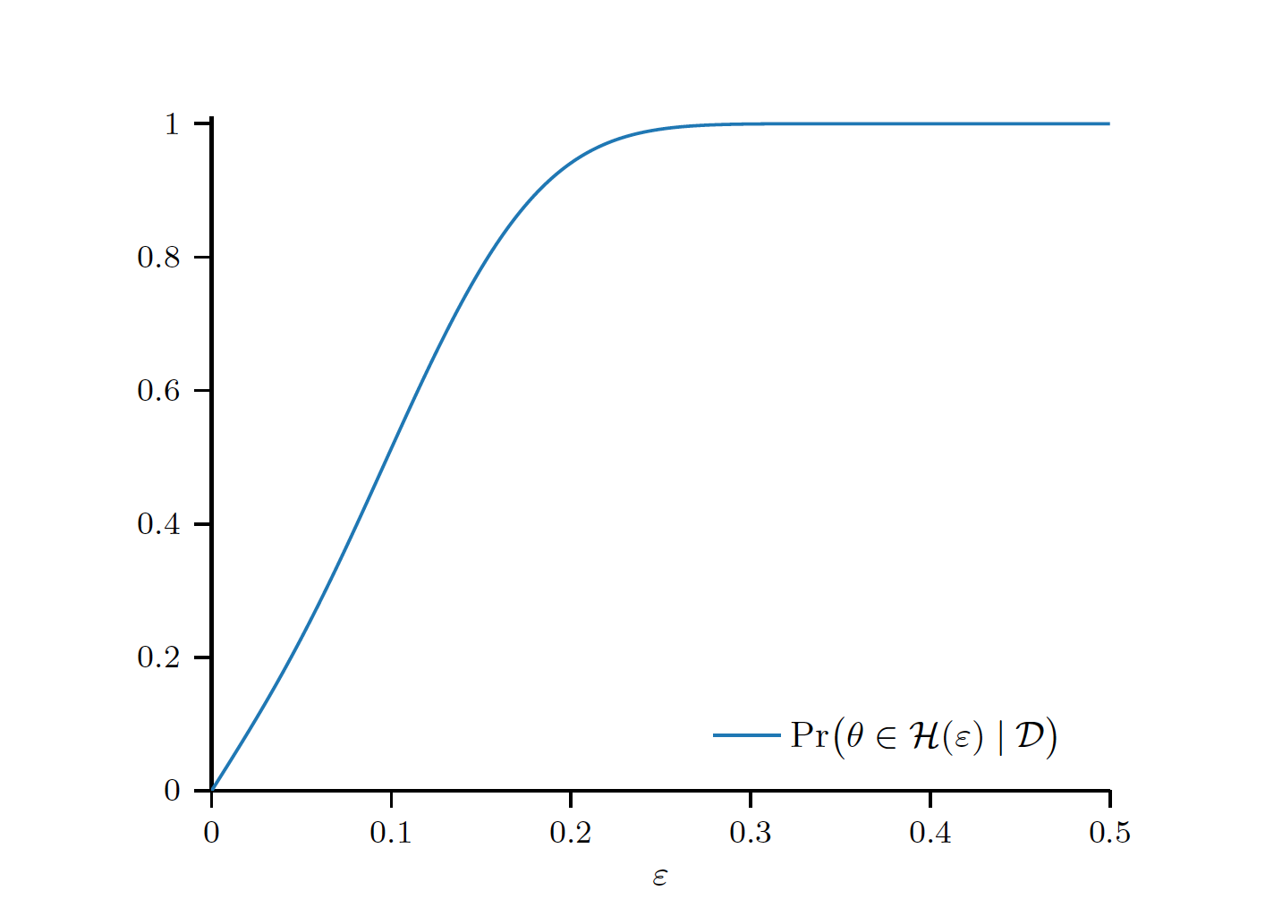
\[Pr(\theta=\frac{1}{2}|\mathcal{D})=\int_{\frac{1}{2}}^{\frac{1}{2}}{p(\theta|\mathcal{D})}d{\theta}=0\]One option would be to consider a parameterized family of hypothesis of the form
\[\mathcal{H}{(\epsilon)}=(\frac{1}{2}-\epsilon, \frac{1}{2}+\epsilon)\]Hypothesis Testing - Frequentist
We will create a so-called “null hypothesis” $\mathcal{H}_0$ that serves to define what “typical” data may look like assuming that hypothesis.
For example, for reasoning about the fairness of a coin, we may choose the natural null hypothesis $\mathcal{H}_0:\theta=\frac{1}{2}$. Now we can use the likelihood
\[Pr(\mathcal{D}|\theta=\frac{1}{2})=Pr(x|n,\theta=\frac{1}{2})\]The classical procedure is then to define a statistic summarizing a given dataset $s(\mathcal{D})$ in some way. An example for coin flipping would be the sample mean $s(\mathcal{D})=\hat{\theta}=\frac{x}{n}$.
We now compute a so-called $\color{orangered}{\textbf{critical set }C(\alpha)}$ with the property
\[Pr(s(\mathcal{D})\in\color{orangered}{C(\alpha)}\color{b}|\mathcal{H}_0)=1-\alpha\]where $\alpha$ is the $\color{orangered}{\textbf{significance level}}$ of the test.
The interpretation of the critical set is that the statistic computed from datasets generated assuming the null hypothesis “usually” have values in this range.
The most critical point here is that $\color{orangered}{\textbf{critical set }C(\alpha)}$ can be calculated based on $\mathcal{H}_0$ without any information from given dataset $\mathcal{D}$.
Finally, we can compute the statistic for a particular set of observed data $s(\mathcal{D})$ and determine whether it lay inside the critical set $\color{orangered}{C(\alpha)}$ we have defined.
(1) If so, the dataset $\mathcal{D}$ appears typical for datasets generated from the null hypothesis.
(2) If not, the dataset appears unusual, in the sense that data $\mathcal{D}$ generated assuming the null hypothesis would have such extreme values of the statistic only a small portion of the time $(100\alpha)$%. IN THIS CASE, you “reject” the null hypothesis $\mathcal{H}_0$ with significance $1-\alpha$.
Hypothesis Testing - p value
A $p$-value is actually the minimum $\alpha$ for which you would reject the null hypothesis using this procedure.
That is the probability that we would observe results as extreme as those in our dataset, as measured by the chosen statistic, if the null hypothesis were true!
For example, in coin flips example, if we have defined certain $p$-value, then we can know like 15heads/20flips is the boundary. Hence, $p$-value will be calculated based on probability summing up from 16/20, 17/20, 18/20, 19/20, 20/20.
Summarizing Distributions - Bayesian
Here, the commonly considered problem is interval summarization, where we provide an interval $(l,u)$ indicating plausible values of the parameter $\theta$ in light of the observed data.
Then, we introduce the concept $\color{orangered}{\textbf{Credible Interval}}$ such that $\theta\in(l,u)$ is “large” (say, has probability $\alpha$):
\[Pr(\theta\in(l,u)|\mathcal{D})=\int_{l}^{u}p(\theta|\mathcal{D})d{\theta}=\alpha\]then we call $(l,u)$ an $\color{orangered}{\alpha-\textbf{Credible Interval}}$ for $\theta$. We have that $\mathcal{H}(\epsilon=0.1)=(0.4,0.6)$ is a 50%-creidible interval for the bias of the coin, and $\mathcal{H}(\epsilon=0.2)=(0.3,0.7)$ is a 95%-credible interval.
Summarizing Distributions - Frequentist
First we are going to define a function $\text{CI}(\mathcal{D})$ that will map a given dataset $\mathcal{D}$ to an interval $(l,u)=\text{CI}(\mathcal{D})$. Now we consider repeating the following experiment:
- collect data $\mathcal{D}$
- compute the interval $(l,u)=\text{CI}(\mathcal{D})$
- state $\theta\in(l,u)$
In the limit of infinitely many repetitions of this experiment, if the final statement is true with probability $\alpha$, then the procedure $\text{CI}(\mathcal{D})$ is called an $\alpha$-confidence interval procedure, and we will write $\text{CI}(\mathcal{D;\alpha})$.
The correct interpretation of above $\color{orangered}{\textbf{confidence interval}}$ is that from so many experiment generated datasets $\mathcal{D}$, there are 100(1-$\alpha$)% $\text{CI}(\mathcal{D;\alpha})$ can contain estimated parameter $\theta$.
1.4 Decision Theory
Point Estimation
In a sense, the posterior contains all information about $\theta$ that we care about. However, the process of inference will often require us to use this posterior to answer various questions. For example, we might be compelled to choose a single value $\hat{\theta}$ to serve as point estimate of $\theta$. To a Bayesian, the selection of $\hat{\theta}$, and in different contexts, we might want to select different values to report.
Decision Theory - Bayesian
- Parameter Space $\Theta$
- Sample Space $\mathcal{X}$
- Action Space $\mathcal{A}=\Theta$
- Decision Rule as a function $\delta:\mathcal{X}\rightarrow{\mathcal{A}}$
- Loss Function $L:\Theta\times{\mathcal{A}}\rightarrow{\mathbb{R}}$
The value $L(\theta,a)$ summarizes “how bad” an action $a$ was if the true value of the parameter was revealed to be $\theta$. Larger losses represent worse outcomes.
Given our observed data $\mathcal{D}$, we find the posterior $p(\theta|\mathcal{D})$, which represents our current belief about the unknown parameter $\theta$. Given a potential action $a$, we may define the posterior expected loss of $a$ by averaging the loss function over the unknown parameter:
\[{\rho}(p(\theta|\mathcal{D}),a)=\mathbb{E}[L(\theta,a)|\mathcal{D}]=\int_{\Theta}L(\theta,a)p(\theta|\mathcal{D})d{\theta}\]Hence, we want to minimize the posterior expected loss with
\[\delta^{*}(\mathcal{D})=\arg \min_{a\in{\mathcal{A}}}{\rho}(p(\theta|\mathcal{D}),a)\]A similar analysis shows that the Bayes estimator for the absolute deviation loss $L(\theta,\hat{\theta})=|\theta-\hat{\theta}|$ is the posterior mean.
The Bayes estimators for a relaxed 0-1 loss:
\[L(\theta,\hat{\theta};\epsilon) \color{b}{ = \begin{cases} 0\ \ \ |\theta-\hat{\theta}|<\epsilon \\ 1\ \ \ |\theta-\hat{\theta}|\geq\epsilon \end{cases}}\]converge to the posterior mode for small $\epsilon$.
The posterior mode also called the $\color{orangered}{\textbf{maximum a posterior(MAP)}}$ estimate of $\theta$, which is written as $\hat{\theta}_{\text{MAP}}$.