Machine Learning Theory
view on github- 1. Learning Problem
- 2. Linear Model
- 3. Overfitting
- 4. Validation
- 5. Three Principles
- 6. Estimating Probabilities from Data
Similar Courses
Recommended Books
- Matrix Cookbook
- Learning From Data (Color)
- Learning From Data (2012)
- Computer Age Statistical Inference
1. Learning Problem
1.1 Mathematical Notation
- unknown target function$f:\mathcal{X}\rightarrow\mathcal{Y}$
- training data $\mathcal{D}$
- hypothesis set $\mathcal{H}$
- learning algorithm $\mathcal{A}$
- learned hypothesis $\mathcal{H}$, and $\mathcal{H}\ni g\approx{f}$
$\mathcal{H,A}$ will be called as learning model, this is what we can control.
1.2 Perceptron
Input $\mathcal{X}\in\mathbb{R}^n$ ($\mathbb{R}^{n}$ is the $n$-dimensional Euclidean space). Output $\mathcal{Y}\in {+1,-1}$. Give a sign function
\[h(\mathbf{x})= \begin{cases} +1\ \ if\sum_{i=1}^{2}w_{i}x_{i}-b>0 \\ -1\ \ otherwise \end{cases}\]which can also be expressed in this way:
\[h(\mathbf{x})=sign((\sum_{i=1}^{n}w_{i}x_{i})+b)\]To simplify the noation of the perceptron formula, we will treat the bias $b$ as a weight $w_0=b$ and merge it with the other weights into one vector $\mathbf{w}=[w_0,w_1,\cdots,w_n]^{T}$,where $^{T}$ denotes the transpose of a vector, so $\mathbf{w}$ is a column vector. We also treat $\mathbf{x}$ as a column vector and modify it to become $\mathbf{x}=[x_0,x_1,\cdots,x_n]^T(where\ x_0=1)$, therefore $\mathbf{x}=(x_1, x_2,\cdots,x_n)\in\mathbb{R}^{n}$
With such convention, we will have
\[\mathbf{w}^{T}\mathbf{x}=\sum_{i=0}^{d}w_ix_i\]Tips:
\[\mathbf{w}^T\mathbf{x}=[w_0,w_1,\cdots,w_n] \left[ \begin{matrix} x_0\\ x_1\\ .\\ .\\ .\\ x_n \end{matrix} \right] = w_0x_0+w_1x_1+\cdots+w_nx_n=\sum_{i=0}^{n}w_ix_i\]Finally, we will get
\[h(\mathbf{x})=sign(\mathbf{w}^T\mathbf{x})\]
1.3 Perceptron Learning Algorithm(PLA)
We will use iterative method to find $\mathbf{w}$. At iteration $t$, where $t=0,1,2,\cdots$, there is a current value of the weight vector, call it $\mathbf{w}(t)$. Then the algorithm will pick one of misclassified examples, called $(\mathbf{x}(t),y(t))$, and uses it to update $\mathbf{w}(t)$. And the update rule is
\[\mathbf{w}(t+1)=\mathbf{w}(t)+y(t)\mathbf{x}(t)\]Tip1: $y(t)$ and $\mathbf{x}(t)$ are actully $y_{n(t)}$, $\mathbf{x}_{n(t)}$ in short.
Tip2: $y(t)$ and $\mathbf{x}(t)$ is a point from training data set $\mathcal{D}={(\mathbf{x_1}, y_1), (\mathbf{x_2}, y_2),\cdots,(\mathbf{x_i}, y_i),\cdots,(\mathbf{x_n}, y_n)}$
Intution: suppose $(\mathbf{x},y)\in\mathcal{D}$ is a misclassified training example and $y=+1$
- $\mathbf{w}^T\mathbf{x}$ is negative
- After updating $\mathbf{w}’=\mathbf{w}+y\mathbf{x}$
- $\mathbf{w}’^T\mathbf{x}=(\mathbf{w}+y\mathbf{x})^T\mathbf{x}=\mathbf{w}^T\mathbf{x}+y\mathbf{x}^T\mathbf{x}$ is less negative that $\mathbf{w}^T\mathbf{x}$
- This will make $\mathbf{w}^T\mathbf{x}$ closer to 0.
2. Linear Model
2.1 Linear Regression
Linear Models:
\[h(\mathbf{x})= \mathbf{some\ function\ of\ w^{T}x}\] \[\mathbf{x}= \left[ \begin{matrix} 1\\ x_1\\ .\\ .\\ x_d \end{matrix} \right]\]where $\mathcal{X}=\mathbb{R}^d$ and y=$\mathbb{R}$. For linear models, we use squared error
\[\begin{aligned} E_{in}(h)&={\frac{1}{n}\sum_{i=1}^{n}(h(\mathbf{x}_i)-y_i)^2 }\\ &={\frac{1}{n}\sum_{i=1}^{n}(h(\mathbf{x}_i)-y_i)^2 }\\ &=\frac{1}{n}||\mathbf{Xw-y}||^2 \\ &= \frac{1}{n}(\mathbf{Xw-y})^T(\mathbf{Xw-y}) \end{aligned}\]
To Minimize the Error: We will find the gradient, and set it equal to zero. By solving the equation, we will need to check that the solution is a minimum. Following are concrete procedure:
\[\begin{aligned} E_{in}(\mathbf{w})&= \frac{1}{n}(\mathbf{Xw-y})^T(\mathbf{Xw-y})\\ &=\frac{1}{n}((\mathbf{Xw})^T-\mathbf{y}^T)(\mathbf{Xw-y})\\ &=\frac{1}{n}(\mathbf{w^T{X^T}Xw-2w^TX^Ty+y^Ty }) \end{aligned}\]Therefore, the gradient will be
\[\nabla_{\mathbf{w}}E_{in}(\mathbf{w})=\frac{1}{n}(2\mathbf{X^TXw}-2\mathbf{X^Ty})\]The Optimized $\mathbf{w^{*}}$
\[\nabla_{\mathbf{w}}E_{in}(\mathbf{w^{*}})=\frac{1}{n}(2\mathbf{X^TXw^{*}}-2\mathbf{X^Ty})=0\]The formula above equals to 0
\[\begin{aligned} 2\mathbf{X^TXw^{*}}-2\mathbf{X^Ty}&=0\\ \mathbf{X^TXw^{*}}&=\mathbf{X^Ty}\\ \mathbf{w^{*}}&=\mathbf{(X^TX)^{-1}X^Ty} \end{aligned}\]Another thing we need do is to check the second derivative of $\mathbf{w}$
\[H_{\mathbf{w}}E_{in}(\mathbf{w})=\frac{1}{n}(2\mathbf{X^TX})\]Here, $H_{\mathbf{w}}E_{in}(\mathbf{w})$ is semidefinite.
2.2 Logistic Regression
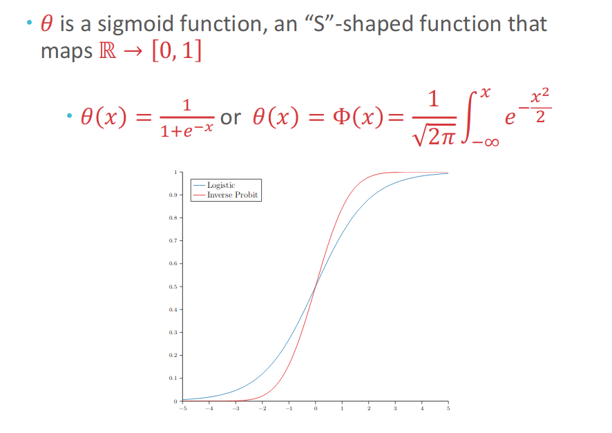
We will use new sigmoid function, $h(\mathbf{x})=\theta(\mathbf{w^Tx})$, $\theta$ is a function which show the probability with range [0,1].
Observation are still binary: $y_i=\pm1$. And our goal is to learn $f(\mathbf{x})=P(y=+1|\mathbf{x})$ (This means that we need to give a probability of $\mathbf{x}$ being $+1$). Therefore, we can rewrite the target goal $f(\mathbf{x})=P(y=+1|\mathbf{x})$ as
\[P(y|\mathbf{x})= \begin{cases} f(\mathbf{x}), & for\ y=+1\\ 1-f(\mathbf{x}), & for\ y=-1 \end{cases}\]
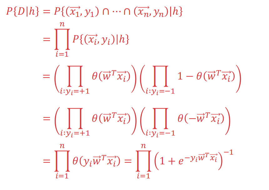
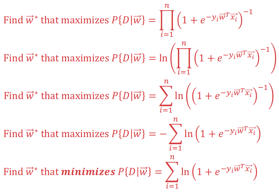
With settling the model function, we need to find a good hypothesis to measure the error. Some hypothesis is good if the probability of the training data $\mathcal{D}$ given by $h$ is high(which measures how our function give probability to). Therefore, we use Cross Entropy function:
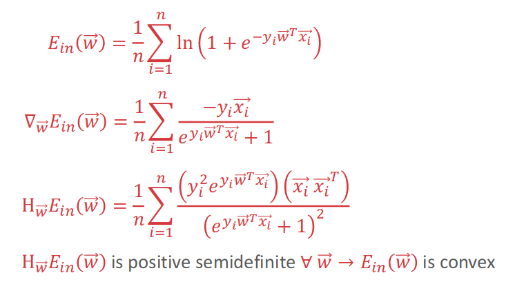
\[E_{in}(\mathbf{w})=\frac{1}{n}{\sum_{i=1}^{n}\ln{(1+e^{-y_i\mathbf{w^Tx_i}})}}\]Following figures will use Probability Union to explain how cross entropy function is got from mathematical induction:
With maximization of above probability union
To minimize above probability function, we introduce Gradient Descent approach. First, we shuold know that cross_entropy is a convex function. After getting the Hessian Matrix with positive semidefinite, we know that Cross-Entropy function is convex.
Then we introduce the Gradient Descent Intution to do such thing.
Suppose current location $\mathbf{w}(t)$ and we get a small step of size $\eta$ in the direction of a unit vector $\hat{v}$. Then we want to move some distance $\eta$ in the “most downhill” direction possible $\hat{v}$
\[\mathbf{w}(t+1)=\mathbf{w}(t)+\eta\hat{v}\]After that, we want to fix $\eta$ and choose $\hat{\mathbf{v}}$ to maximize the decrease in $E_{in}$ after making the update $\mathbf{w}(t+1)=\mathbf{w}(t)+\eta\hat{v}$. Therefore, we can get \(\Delta{E_{in}}(\hat{v})=E_{in}(\mathbf{w}(t)+\eta\hat{v})-E_{in}(\mathbf{w}(t))\) What we want to do here is to maximum the decreation here to Minimum the $E$ function.
\[\begin{aligned} \Delta{E_{in}}(\hat{v})&=E_{in}(\mathbf{w}(t)+\eta\hat{v})-E_{in}(\mathbf{w}(t))\\ &{\approx} (E_{in}(\mathbf{w}(t))+\eta\hat{v}^{\mathbf{T}}\nabla_{\mathbf{w}}{E_{in}(\mathbf{w}(t)))}-E_{in}(\mathbf{w}(t)) \\ &{\approx}\eta\hat{v}^{\mathbf{T}}\nabla_{\mathbf{w}}{E_{in}(\mathbf{w}(t))}\\ &\geq{-\eta||\nabla_{\mathbf{w}}{E_{in}(\mathbf{w}(t))||}} \end{aligned}\]
The explanation for the last line here is
\[\mathbf{a}\cdot\mathbf{b}=-|\mathbf{a}|\cdot|\mathbf{b}|\]And the explanation for second line here(Gradient):
- Knowing that $\mathbf{x,\ w}\in{\mathbb{R}^{d+1}}$, and means that $\mathbf{x,\ w}$ has d+1 dimensions.
- Thus,
- And $\mathbf{v}$ is a vector with same dimensions as $\mathbf{w}$
- First Order Taylor Expansion:
- Thus, the optimial direction should be
- Intution for Step
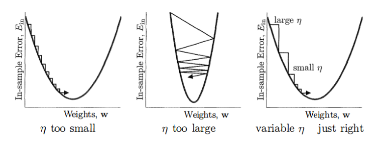
A simple heuristic can do this. The gradient close to minimum is small and away from minimum can be large. Thus, we can set
\[\eta_{t}=\eta_{0}||\nabla_{\mathbf{w}}E_{in}(\mathbf{w}(t))||\]Finally, we get
\[\begin{aligned} \mathbf{w}(t+1)&=\mathbf{w}(t)+\eta_t\hat{v^{*}_{t}}\\ &=\mathbf{w}(t)+(\eta_{0}||\nabla_{\mathbf{w}}E_{in}(\mathbf{w}(t))||)(-\frac{\nabla_{\mathbf{w}}E_{in}(\mathbf{w}(t))}{||\nabla_{\mathbf{w}}E_{in}(\mathbf{w}(t))||})\\ &= \mathbf{w}(t)-\eta_0\nabla_{\mathbf{w}}E_{in}(\mathbf{w}(t)) \end{aligned}\]
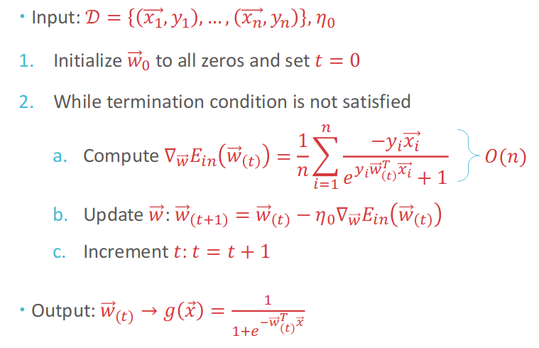
- Gradient Descent Algorithm
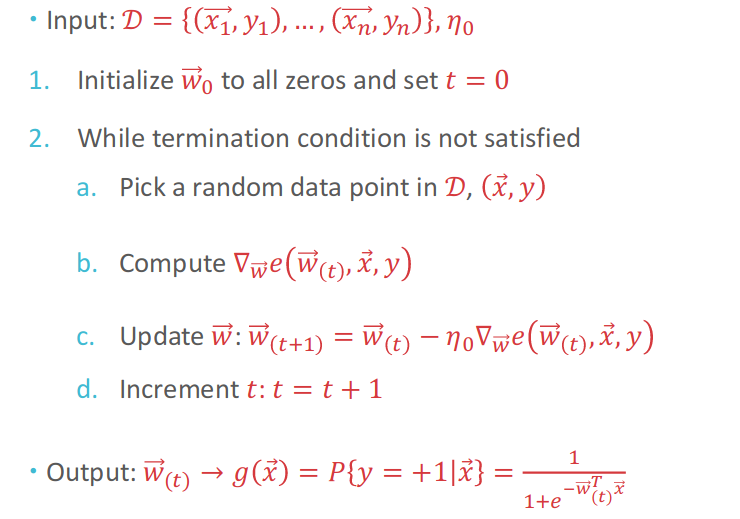
- SGD(Stochastic Gradient Descent)
3. Overfitting
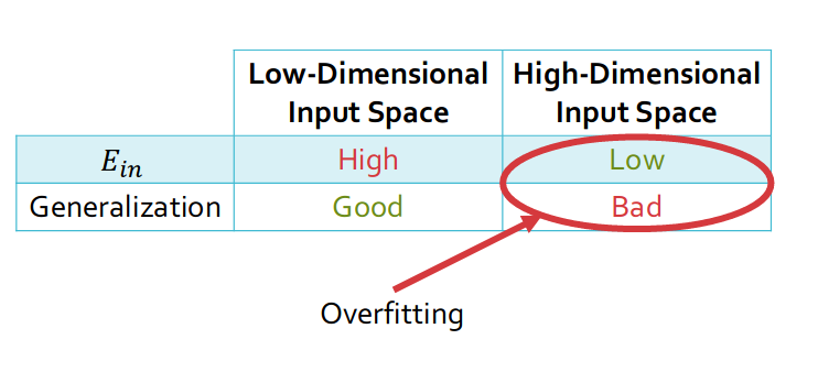
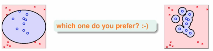
With High-Dimensional Input Space, sometimes it will cause low in-sample error and bad generalization, which can be demonstrated in following figure:
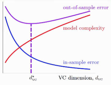
Also Error and Model Complexity’s relationship can be demonstrated in following ways:
To understand the overfitting, we need to know the cause for Overfitting:
- Too complexity: High kth-Order=>High VC-dimension: drive too fast
- Noise: bumpy road
- Too limited data: not familiar with road conditions
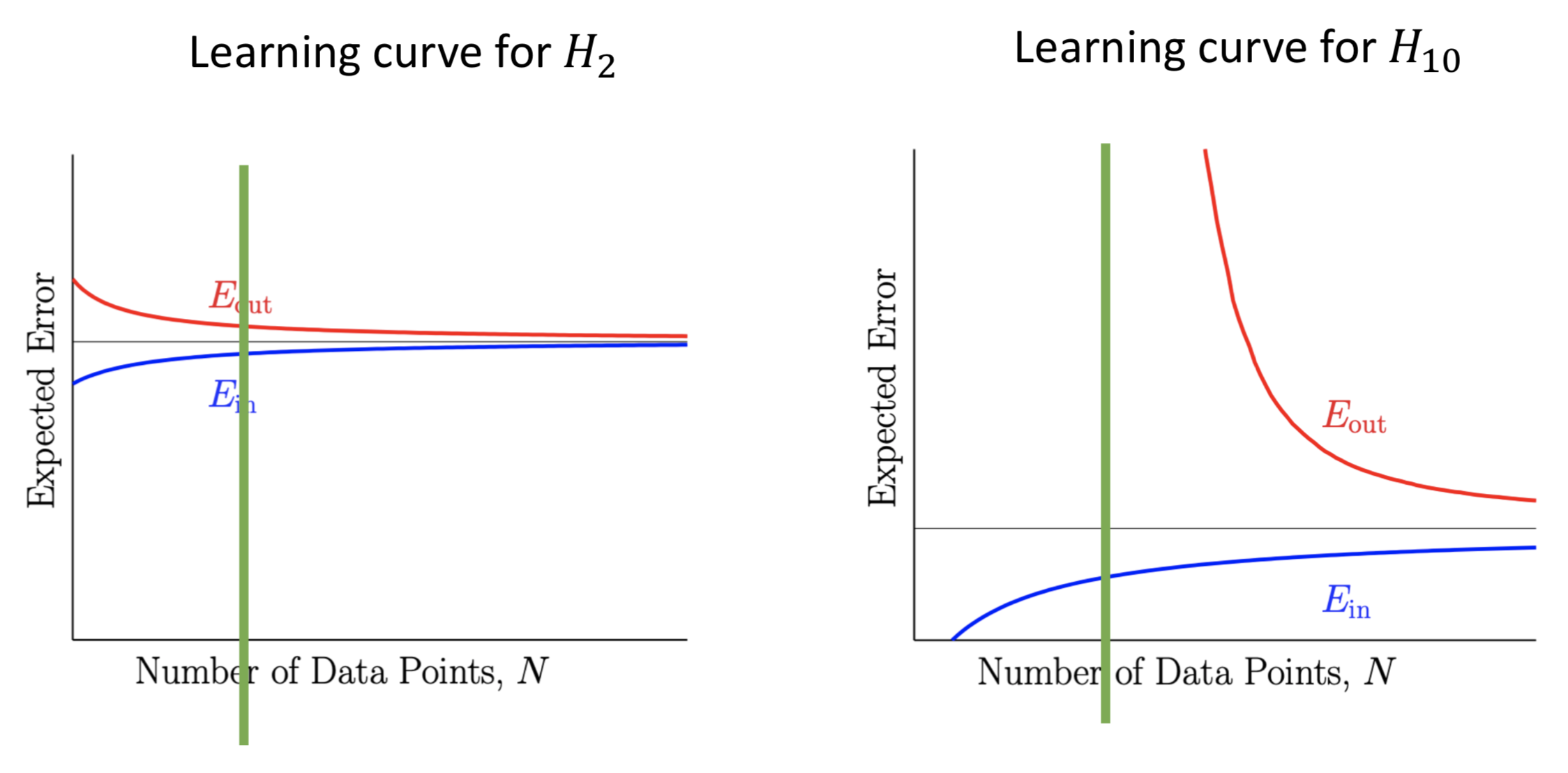
The figure above shows that in the right of green line area, which means we have limited data samples. The complex model($\mathcal{H_{10}}$) have larger $E_{out}$ than simple model ($\mathcal{H_{2}}$).
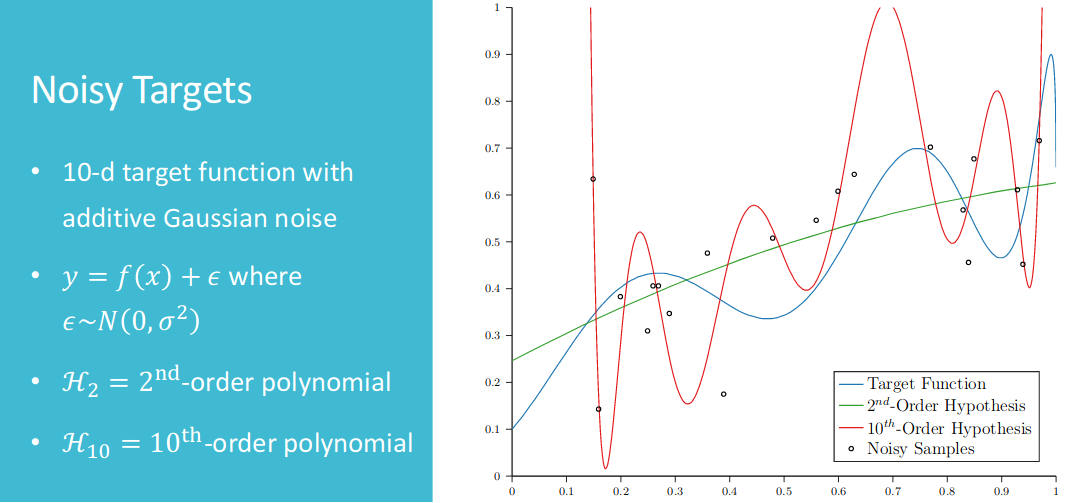
Before getting more data, the simple model will have better effect. Following first figure is the comparison between lower order and higher order polynomial.
- Less Data with 20 Points
- More Data with 100 Points
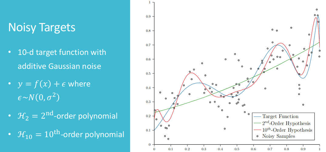
After increasing number of data, the complex model($\mathcal{H_{10}}$) wins. And to solve overfitting problems, we may want to (1)start from simple model;(2)data cleaning / pruning; (3)data hinting; (4)regularization; (5)validation.
4. Validation
4.1 Model Selection (Not Single Hypothesis Anymore)
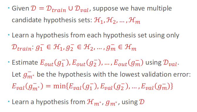
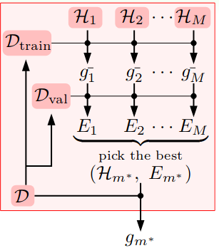
Tips: At here, $\mathcal{H}_{val}$ are formed up from many signle hypothesis from multiple hypothesis sets, and we are going to pick a best hypothesis set.
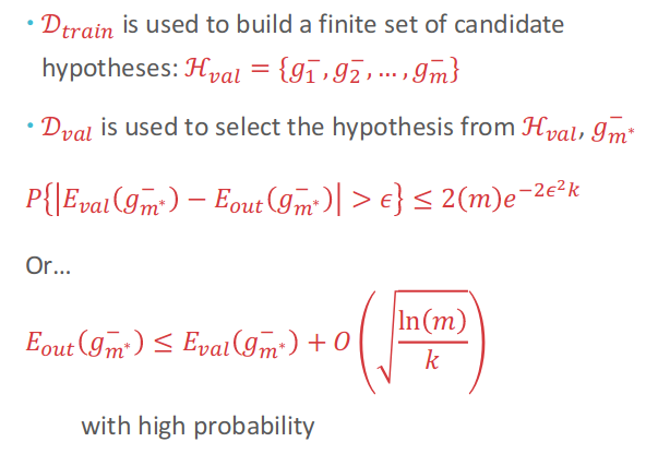
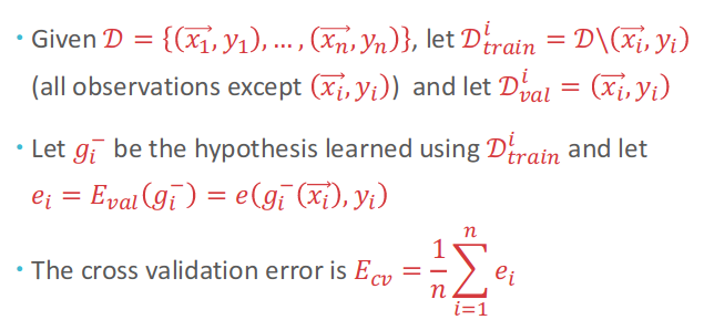
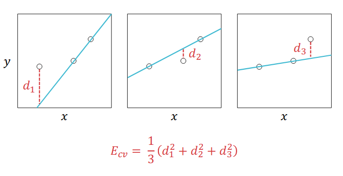
4.2 Leave-one-out cross validation(LOOCV)
Cross here means that this data point can be training data and validation data. And $E_{cv}$ is almost an unbiased estimator of $E_{out}(g)$.
Making an concrete example for calculating LOOCV Error:
Model selection
- For each hypothesis set, we need to run $n$ points to get its error.
- Then, just like the validation data set above, we can just pick a best hypothesis $g^{-}{m^{*}}$ which comes from hypothesis set $\mathcal{H}{m^{*}}$
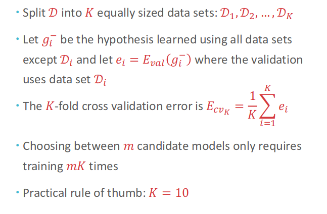
4.3 K-fold cross validation
5. Three Principles
5.1 Occam ‘s Razor
An explanation of the data should be made as simple as possible, but no simpler. ——Albert Einstein
Entities must not be multiplied beyond necessity. ——William of Occam
Occam’s Razor for learning: The simplest model that fits the data is also the plausible.
5.2 Simple Models
Simple Hypothesis $h$: Few parameters. And Simple Model $\mathcal{H}$: contain small number of hypotheses(slow growth function). The connection between simple hypothesis and simple model is that if we only have $2^{l}$ hypotheses, then we only need $l$ bits to represent each model.For example, constrain with weight be smaller than 2 for 2-dimensions positive integer, then we have at most 4 hypotheses with 2 parameters. Therefore,
\[small\ \Omega(\mathcal{H})\rightarrow{small\ Omega(h)}\]Case Study #1:
Suppose I tell you that I have found a $10^{th}$-order polynomial that perfectly fits my dataset of 10 points. Should you believe that the true function is a $10^{th}$-order polynomial? The Answer is no! Since $10^{th}$-order polynomial function can always fits 10 points. And suppose I tell you I have found a line that perfectly fits my dataset of 10 points? The answer will be yes!
Axiom of Non-falsifiability: If an experiment has no chance of falsifying a hypothesis, then the result of that experiment provides no evidence one way or the other for the hypothesis.
5.3 Sampling Bias
Case Study #2:
(1) Presidential Story: 1948 US President election => Truman versus Dewey
(2) Trump versus HillaryTherefore, we need Data and Testing both iid from $\mathcal{P}$. If not from the same distribution, we will have VC Fails
5.4 Data Snooping
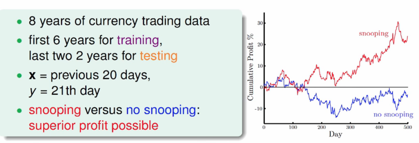
(1) Red line shows the result when we compute $z$ with 8 years data(train & test)
(2) Blue line shows the result when we compute $z$ with 6 years training data and normalize test data with mean and variance from training data.
To avoid Data Snooping, we need to avoid several following things:
- Visualize data => careful about your brain’s model complexity.
- “If you torture the data long enough, it will confess.”, which is the phenomena called Data Reuse. Trying different models on the same data set will eventually lead to “success”. Therefore, we need to reuse by computing the combined VC dimension of all models(including what others tried)
- Be Blind: Avoid making modeling decision by data
6. Estimating Probabilities from Data
6.1 MLE (Maximum Likelihood Estimation)
(1) Let $p(y=H)=\theta$, where $\theta$ is the unknown parameter, and all we have is $D$. So, the goal is to choose $\theta$ such taht observed data $D$ is most like likely.
\[\hat{\theta}_{MLE}=\arg{\max_{\theta}} {P(D|\theta)}\]
(2) Formally(MLE principle), Find $\hat{\theta}$ that maximizes the likelihood of the data $p(D|\theta)$.
(3) Goal:
Example: Coin Flipping
\[\begin{aligned} \hat{\theta}_{MLE}&=\arg{\max_{\theta}} {P(D|\theta)}\\ &=\arg{\max_{\theta}}{C_{n}^{n_{H}}\theta^{n_{H}}(1-\theta)^{n-n_{H}}}\\ &= \arg{\max_{\theta}}\ {\log{C_{n}^{n_{H}}} + n_{H}\log{\theta} + (n-n_{H})\log(1-\theta)} \end{aligned}\]Take derivative for above formula, we can get
\[\hat{\theta}_{MLE}=\frac{n_{H}}{n}\]6.2 MAP (Maximum A-Posterior) Estimation
To avoid the randomness of data, you may want to use baysian way to estimate $\theta$. Following is the Baysian Way - Maximum A Posterior(MAP):
\[P(\theta|D) = \frac{P(D|\theta)P(\theta)}{P(D)}{\propto}{P(D|\theta)P(\theta)}\]
- (1) Model $\theta$ as a random variable
- (2) Where $\theta$ is a drown from a distribution
- (3) New, we look at
Tips for notation:
$P(D|\theta)$ : likelihood of the data given the parameters $\theta$
$P(\theta)$ : prior distribution over the parameters $\theta$
$P(\theta|D)$ : posterior distribution over the parameters $\theta$
A useful prior distribution
\[P(\theta|D)=Beta(n_{H}+\alpha, n_{T}+\beta)\]
Beta distribution: $P(\theta)=Beta{(\theta|\alpha, \beta) }= \frac{\theta^{\alpha-1}(1-\theta)^{\beta-1}}{b(\alpha, \beta)}$, where $b(\alpha, \beta)=\frac{\Gamma(\alpha)\Gamma(\beta)}{\Gamma(\alpha+\beta)}$, and note thatGoal: Maximize the posterior distribution $P(\theta|D)$
\[\begin{aligned} \hat{\theta}_{MAP}&=\arg \max_{\theta}\ {P(\theta|D)}\\ &=\arg \max_{\theta}\ \frac{P(D|\theta)P(\theta)}{P(D)}\\ &=\arg \max_{\theta}\ P(D|\theta)P(\theta)\\ \end{aligned}\]
Example: Coin Flipping
Since we know that $P(D|\theta)$ is Binomial Distribution, and we have prior distribution for $P(\theta)$
Hence,
\[\hat{\theta}_{MAP}=\frac{n_{H}+\alpha-1}{n+\alpha+\beta-2}\]Advantages:
(1) as $n$ approach infinity, MAP Estimation will approach MLE.
(2) MAP is a great estimator if prior belief exists and is accurate
Disadvantages:
(1) If $n$ is small, it can be very wrong if prior belief is wrong
(2) Also we have to choose a reasonable prior
Posterior Mean: Note that MAP is only one way to get an estimator for $\theta$. There is much more information in $P(\theta|D)$. So, instead of the maximum as we did with MAP, we can use the posterior mean (and even its variance).
\[\hat{\theta}_{\text{MEAN}}=E[\theta, D]=\int_{\theta}\theta{p(\theta|D)}d\theta\]
Posterior Predictive: So far, we talked about modeling and estimating parameters. But in machine learning, we actually interested in predictions. To directly estimate label $y$ from the given data, we can use the posterior predictive distribution.
In our coin tossing example, this is given by: (since we know that \(p(y=H|\theta,D)=\theta\) in the coin flipping).
\[\begin{aligned} p(y=H|D)&=\int_{\theta}p(y=H, \theta |D)d\theta\\ &=\int_{\theta}p(y=H|\theta,D)p(\theta|D)d\theta\\ &=\int_{\theta}\theta{p(\theta|D)}d\theta \end{aligned}\]In general, the posterior predictive distribution is ($\mathbf{x}$ is test input, and $\theta$ means the $\mathbf{w}$ or the parameters in model)
\[\begin{aligned} p(y|D,\mathbf{x})&=\int_{\theta}p(y,\theta|D,\mathbf{x})d\theta\\ &=\int_{\theta}p(y|D, \mathbf{x}, \theta)\cdot{p(\theta|D,\mathbf{x})}d\theta\\ &=\int_{\theta}p(y|D, \mathbf{x}, \theta)\cdot{p(\theta|D)}d\theta \end{aligned}\]
6.3 MLE and MAP for discrimitive supervised learning
Usually, there are two assumptions in discrimitive supervised learning:
(1) $\mathbf{x}_i$ are known, => $\mathbf{x}_i$ independant of the model parameters $\mathbf{w}$, hence
\[p(X|\mathbf{w})=p(X)\]and
\[p(\mathbf{w}|X)=p(\mathbf{w})\](2) $y_i$ are independent ghven the input features $\mathbf{x}_i$ and $\mathbf{w}$
Goal: Estimate $\mathbf{w}$ directly from $D={(\mathbf{x}, y_i)}^{n}_{i=1}$ using the joint conditional likelihood
\[p(\mathbf{y}|X,\mathbf{w})\]
6.3.1 Maximum Likelihood Estimation
Choose $\mathbf{w}$ to maximize the conditional likelihood. (use two assumptions above)
\[\begin{aligned} \hat{\mathbf{w}}_{\text{MLE}}&=\arg \max_{\mathbf{w}} {p(D|\mathbf{w})}\\ &= \arg \max_{\mathbf{w}} {p(\mathbf{y}|X,\mathbf{w})}\\ &= \arg \max_{\mathbf{w}} {\prod_{i=1}^{n}p(y_i|\mathbf{x}_i, \mathbf{w})}\\ &= \arg \max_{\mathbf{w}} {\sum_{i=1}^{n} \log{p(y_i|\mathbf{x}_i, \mathbf{w})} } \end{aligned}\]
6.3.2 Bayesian way to Maximum-a-posterior Estimation
Model $\mathbf{w}$ as a random variable from $p(\mathbf{w})$ and use $p(\mathbf{w}|D)$. Choose $\mathbf{w}$ to maximize the posterior \(p(\mathbf{w}|X,\mathbf{y})\) over $\mathbf{w}$.
\[\begin{aligned} \hat{\mathbf{w}}_{\text{MAP}}&=\arg \max_{\mathbf{w}} {p(\mathbf{w}|X, \mathbf{y})}\\ &=\arg \max_{\mathbf{w}} {p( X,\mathbf{y}|\mathbf{w})\cdot{p(\mathbf{w})}}\\ &= \arg \max_{\mathbf{w}} {p(\mathbf{y}|X,\mathbf{w})\cdot{p(\mathbf{w})}}\\ &= \arg \max_{\mathbf{w}} {\prod_{i=1}^{n}p(y_i|\mathbf{x}_i, \mathbf{w})\cdot{p(\mathbf{w})}}\\ &= \arg \max_{\mathbf{w}} {\sum_{i=1}^{n} \log{p(y_i|\mathbf{x}_i, \mathbf{w})} + \log{p(\mathbf{w})} } \end{aligned}\]
Example: Linear Regression
Model Assumption: $y_i = \mathbf{w}^{\text{T}}\mathbf{x}_i+\epsilon_i \in \mathbb{R}$, where we use the Gussian distribution to model the noise $\epsilon_i \sim N(0,\sigma^2)$
MLE: it is like OLS/squared loss
MAP: Additional Model Assumption, prior distribution (ensure for yourself that the following is a conjuate prior to our likelihood). Then it is like l2-regularization